Excel SUMIF function calculates the sum of a range of cells based on specified criteria. It allows the users to specify a range of cells to be evaluated against criteria for determining which of those cells should be included in the sum, as well as putting a different range of cells to be used in the actual sum.
The syntax of the Excel SUMIF function is as follows:
SUMIF(range, criteria, [sum_range])
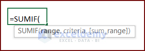
Arguments Explanation:
| Parameter | Data Type | Description | Requirement |
|---|---|---|---|
| range | Range of Cells | The range of cells that you want to evaluate based on criteria. The range can be a single column or row, or multiple columns or rows. | Required |
| criteria | Value or expression | The condition that you want to apply to the range of cells. The criteria can be a value, a cell reference, or an expression that evaluates to a value or cell reference. | Required |
| sum_range | Range of cells | The range of cells that you want to add up. If this argument is omitted, Excel will use the first range argument for the summing operation. The sum_range can be a single column or row, or multiple columns or rows, but must be the same size as range. | Optional |
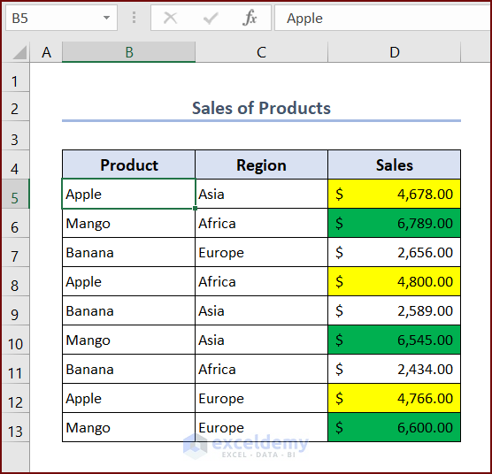
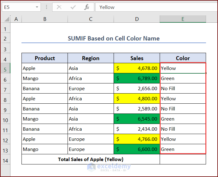
For this example, consider a dataset that contains the names of the products, their regions, and their total sales amount. The cells containing the sales amount have different colors based on the product names. Those colors will be used for criteria in the SUMIF functions.
Method 1 – Apply Excel SUMIF Function with Cell Color Code
We can apply the Excel SUMIF function with cell color code as a criteria, which you can get via the GET.CELL function in Name Manager.
Steps:
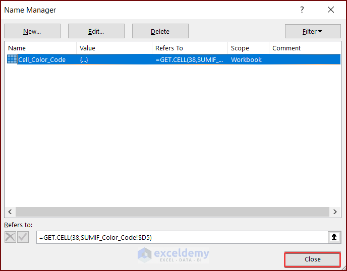
- Select cell D5 and go to the Formulas tab, then choose Name Manager.
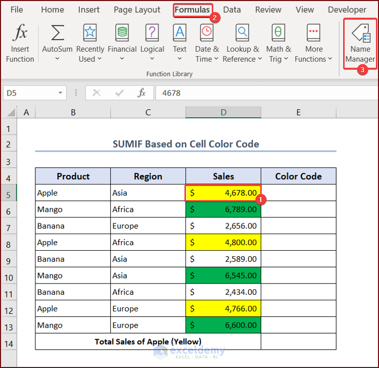
- A new window will pop up named New Name.
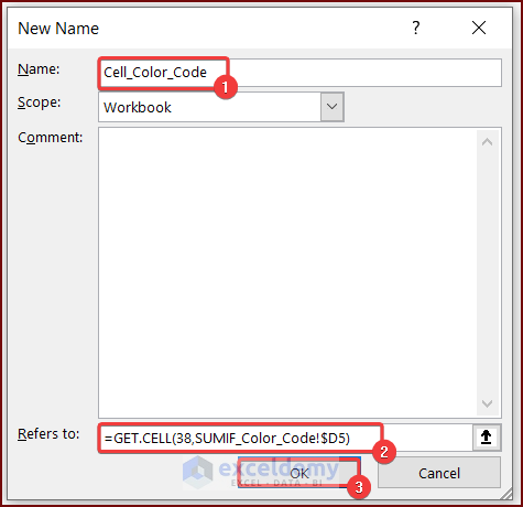
- Insert Cell_Color_Code as the Name.
- Put this formula into the reference box:
=GET.CELL(38,SUMIF_Color_Code!$D5)
- Press OK to confirm.
- Now close the Name Manager.
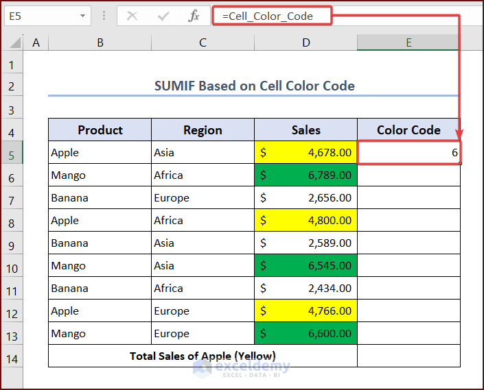
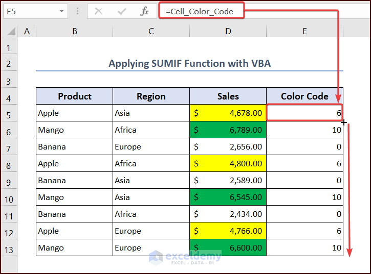
- Put this formula in cell E5:
=Cell_Color_Code
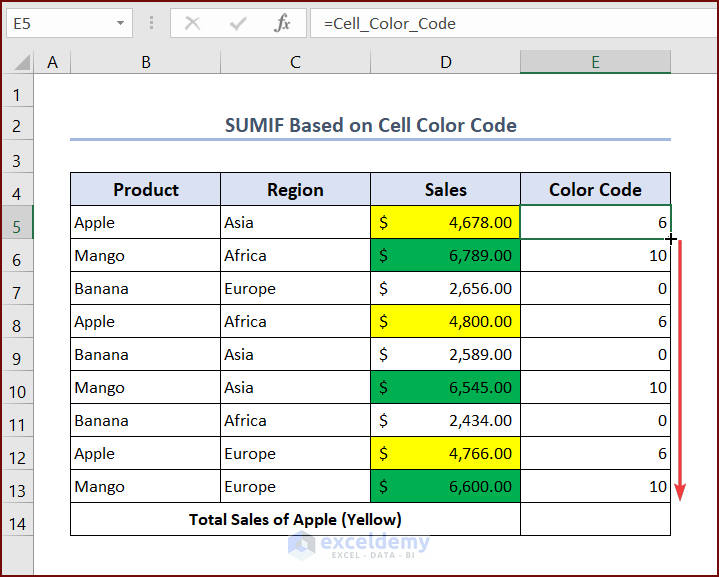
- Use Fill Handle to AutoFill data throughout the range E5:E13.
- Type this formula in cell E14:
=SUMIF(E5:E13,6,D5:D13)- Press Enter and you will see the total sales amount of apples in cell E14.
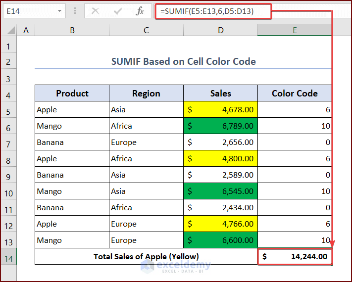
The SUMIF function will return the sum of specific cells in range D5:D13 that match the criteria (6) in the corresponding cells of range E5:E13.
If the GET.CELL function is BLOCKED in your worksheet, you need to enable Excel 4.0 macro in your workbook:
- Go to Developer >> Macro Security >> Macro Settings.
- Check the box that says Enable Excel 4.0 macros when VBA macros are enabled.
- Press OK to save changes.
Read More: How to Sum If Cell Contains Number and Text in Excel
Method 2 – Use Excel SUMIF Function with Cell Color Name
For this method to work, you’ll need to manually input the color name.
Steps:
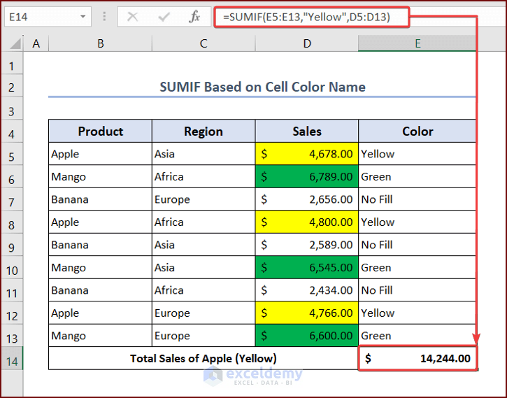
- Select cell E14 and put in the following formula:
=SUMIF(E5:E13,"Yellow",D5:D13)- Press Enter and you will see the total sales amount of apples.
Read More: How to Sum If Cell Contains Number in Excel
Method 3 – Create a VBA Code to Get a Sum Based on Cell Color
Steps:
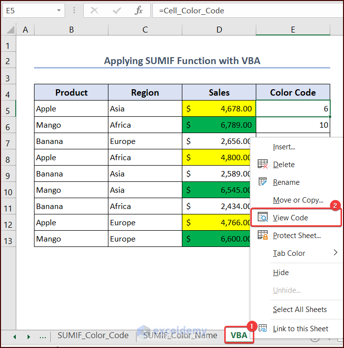
- Get the color codes of the cells using the CELL function from the Name Manager. You can follow Method 1 to do so.
- Right-click on your worksheet and select View Code.
 Go to Insert, then Module.
- Paste the following code in your VBA Editor and press the Run button or F5 key to run the code.
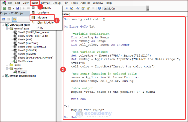
Sub sum_by_cell_color()
On Error GoTo Txt
    'variable declaration
    Dim colorRng As Range
    Dim sumRng As Range
    Dim cell_color, summa As Integer
    'set variable values
    Set colorRng = Sheets("VBA").Range("E5:E13")
    Set sumRng = Application.InputBox("Select the Sales range:", Type:=8)
    cell_color = InputBox("Insert the color code")
    'use SUMIF function in colored cells
    summa = Application.WorksheetFunction.SumIf(colorRng, cell_color, sumRng)
    'show output
    MsgBox "Total sales of the product: $" & summa
    Exit Sub
Txt:
    MsgBox "Not Found"
End Sub
VBA Breakdown
Sub sum_by_cell_color()- Sub indicates a subroutine called sum_by_cell_color.
On Error GoTo Txt- This is an error-handling statement that tells the program to jump to the Txt section if an error occurs.
    Dim colorRng As Range
    Dim sumRng As Range
Dim cell_color, summa As Integer- These are declared variables.
    Set colorRng = Sheets("VBA").Range("E5:E13")
    Set sumRng = Application.InputBox("Select the Sales range:", Type:=8)
cell_color = InputBox("Insert the color code")- These commands set the values of some of the variables. colorRng takes values E5 to E13 from the worksheet called VBA. sumRng and cell_color pick up values from the dialog InputBox.
summa = Application.WorksheetFunction.SumIf(colorRng, cell_color, sumRng)- This uses the SUMIF function from the worksheet to sum the values in the sumRng range that have the same background color as the cell_color value in the colorRng. The result is stored in the summa variable.
MsgBox "Total sales of the product: $" & summa- This MsgBox shows the output.
Exit Sub- This exits the subroutine.
Txt:
    MsgBox "Not Found"
End Sub- This is the error handling section that is triggered if any error occurs. It displays the message “Not Found”.
Method 4 – Use Excel VBA SUMIF to Create a UserForm and Get Sum Based on Cell Color
This section applies the following code in the UserForm that uses the Excel SUMIF function to get a sum based on cell color.
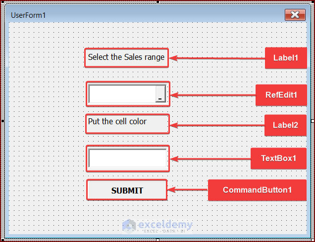
Simply follow the steps below to create the UserForm:
- Go to Insert, then to UserForm.
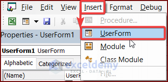
- From the Toolbox, you can choose different controls for your UserForm.
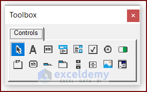
- Insert a few Labels to write instructions.
- Insert a RefEdit that accepts a Range type data and a TextBox that allows a String type data for user input.
- Put a CommandButton to start processing.
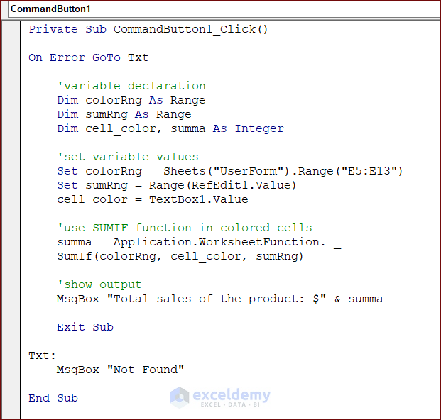
- Double-click on the CommandButton. A new window will open. Enter the following code:
Private Sub CommandButton1_Click()
On Error GoTo Txt
    'variable declaration
    Dim colorRng As Range
    Dim sumRng As Range
    Dim cell_color, summa As Integer
    'set variable values
    Set colorRng = Sheets("UserForm").Range("E5:E13")
    Set sumRng = Range(RefEdit1.Value)
    cell_color = TextBox1.Value
    'use SUMIF function in colored cells
    summa = Application.WorksheetFunction.SumIf(colorRng, cell_color, sumRng)
    'show output
    MsgBox "Total sales of the product: $" & summa
    Exit Sub
Txt:
    MsgBox "Not Found"
End Sub- Run the UserForm and fill in the text boxes to get the results.
VBA Breakdown
Private Sub CommandButton1_Click()- This is the start of a subroutine called CommandButton1_Click. This subroutine is executed when the user clicks on the SUBMIT button on the UserForm.
On Error GoTo Txt- This is an error handling statement that tells the program to jump to the Txt section if an error occurs.
    Dim colorRng As Range
    Dim sumRng As Range
Dim cell_color, summa As Integer- These are declared variables that the function will use for calculations.
Set colorRng = Sheets("UserForm").Range("E5:E13")- This sets the colorRng variable to the range E5:E13 from the worksheet named UserForm.
Set sumRng = Range(RefEdit1.Value)- This sets the sumRng variable to the range selected by the user through the RefEdit in the form.
cell_color = TextBox1.Value- This sets the cell_color variable to the value entered by the user through the TextBox in the form.
summa = Application.WorksheetFunction.SumIf(colorRng, cell_color, sumRng)- This uses the SUMIF function from the worksheet to sum the values in the sumRng range that have the same background color as the cell_color value in the colorRng. The result is stored in the summa variable.
MsgBox "Total sales of the product: $" & summa- This MsgBox shows the output produced by the form.
Exit Sub- This exits the subroutine.
Txt:
    MsgBox "Not Found"
End Sub- If any error occurs, it will trigger this error handling section. It displays a MsgBox that shows the message “Not Found”.
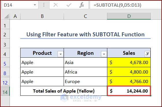
Alternative to SUMIF – Use Filter Feature with SUBTOTAL Function to Sum Colored Cells in Excel
Steps:
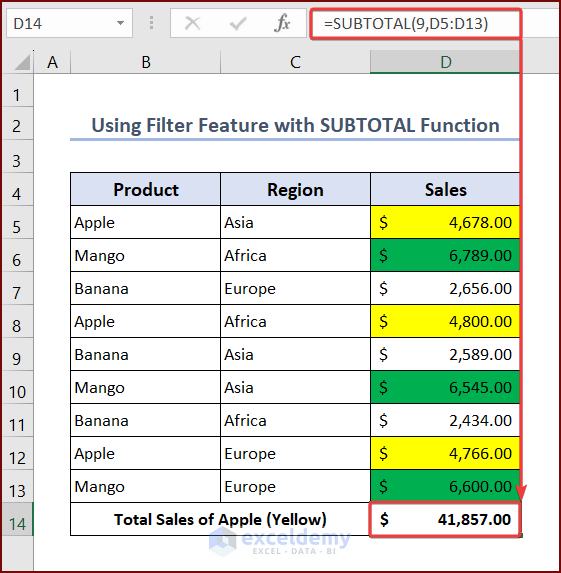
- Select cell D14 and paste the following formula:
=SUBTOTAL(9,D5:D13)- Press Enter and you will see the total sales of all the products.
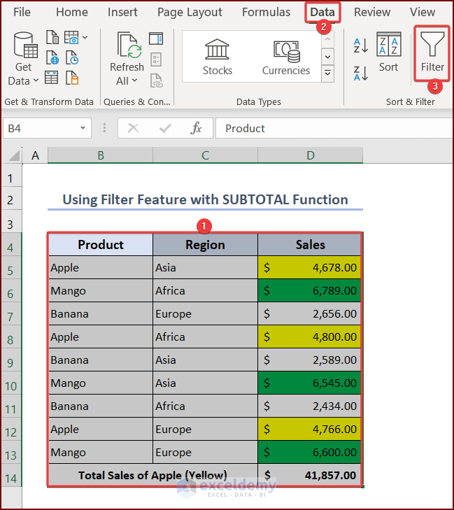
- Select the entire dataset and go to the Data tab, then choose Filter.
- Press the drop-down on the Sales column, then select the Filter icon.
- Click on Filter by color and select the Yellow color.
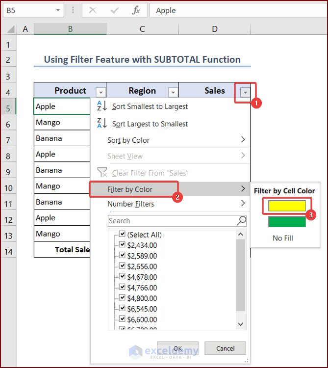
You will see the total sales amount of apples.
Read More: How to Use Excel SUMIF to Sum Values Greater Than 0
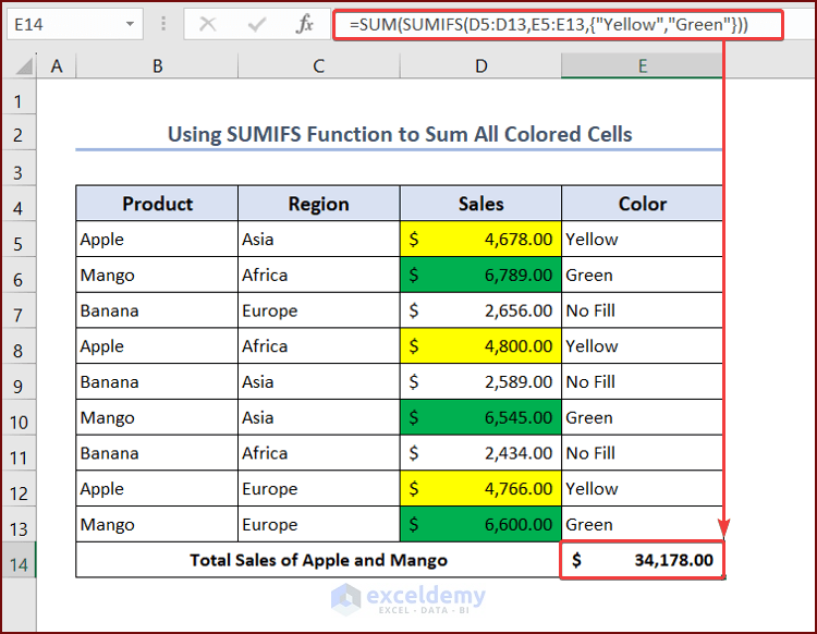
Combine SUM and SUMIFS Functions to Sum All Colored Cells in Excel
You will need to manually spell what colors the cells are in a separate column, like in the example.
Steps:
- Select cell E14 and put the following formula:
=SUM(SUMIFS(D5:D13,E5:E13,{"Yellow","Green"}))- Press Enter and you will see the summation of all colored cells (Yellow and Green).
Note: Press Ctrl + Shift + Enter for older versions of Excel as it acts like an array formula.
Formula Breakdown
- SUMIFS(D5:D13,E5:E13,{“Yellow”,”Green”})
The SUMIFS function will sum the values from range D5:D13 that correspond to the rows where the values in range E5:E13 are either “Yellow” or “Green”. This array formula returns two values as an array; the sum of cells that are Yellow and the sum of cells that are Green.
- SUM(SUMIFS(D5:D13,E5:E13,{“Yellow”,”Green”}))
The SUM function takes the output of the SUMIFS function and returns the final sum of those values.
Alternative: You can also use the combination of SUM and SUMIF functions to sum all the colored cells. You may use the following formula.
=SUM(SUMIF(E5:E13,"Yellow",D5:D13),SUMIF(E5:E13,"Green",D5:D13))Read More: How to Use SUMIF to SUM Less Than 0 in Excel
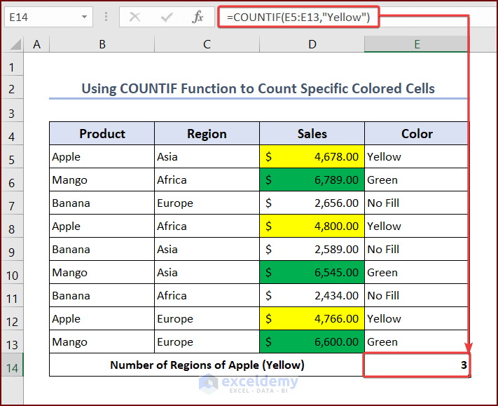
How to Count Specific Colored Cells in Excel Using COUNTIF Function
Steps:
- Select cell E14 and put the following formula:
=COUNTIF(E5:E13,"Yellow")- Press Enter and you will see the number of regions of apples (corresponding cell color is Yellow).
Things to Remember
There are a few things to remember while using Excel SUMIF function based on cell color:
- Use the correct color reference.
- If you don’t use the CELL. functions, you’ll need to have separate cells that manually spell the name, or code them to fetch those values.
- Use the $ sign properly for absolute cell referencing.
- Specify the correct worksheet while applying VBA codes.
Frequently Asked Questions
- Can I use the Excel SUMIF function based on cell color in all versions of Excel?
The ability to use the Excel SUMIF function as indicated in the samples above is available in Excel 2007 and later versions.
- Can I use the Excel SUMIF function based on cell color to sum values in cells with conditional formatting that is based on a formula?
Yes, but you need to use the same formula that is used in the conditional formatting as the criteria in the SUMIF function.
- Can I use the Excel SUMIF function based on cell color to sum values in cells with multiple colors?
No, the Excel SUMIF function based on cell color only works when the cells have one color. If the cells have multiple colors, the function will not work correctly.
Download Practice Workbook
You can download this practice workbook while going through this article.
Related Articles
- Sum If Greater Than and Less Than Cell Value in Excel
- How to Use Excel SUMIF with Greater Than Criterion
- How to Use 3D SUMIF for Multiple Worksheets in Excel
<< Go Back to Excel SUMIF Function | Excel Functions | Learn Excel
Get FREE Advanced Excel Exercises with Solutions!
