Latest Posts From Sajid Ahmed
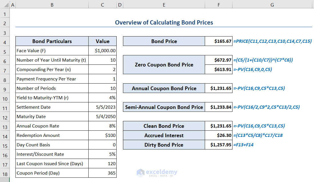
You can determine the present value of a bond with the bond price calculator in Excel. It helps you to assess the fair value of a bond and make correct ...

Below is an overview: Download Practice Workbook Download the Excel file. Use of Excel Calculation Options.xlsm This is the sample ...
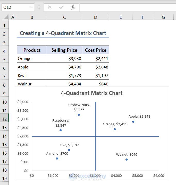
In this article, you’ll learn how to create a Matrix Bubble chart, a 4-Quadrant Matrix chart and a Scatterplot Matrix chart in Excel. In a variety of ...

In this article, you’ll learn how to calculate standard deviation using formula in Excel. We'll calculate both the sample standard deviation and the population ...

This is an overview: Download Practice Workbook Download the Excel files. Excel CSV.xlsm Excel CSV.csv Excel CSV UTF.csv ...

The image below is an overview of using the COUNTIF function with multiple criteria in Excel. Download Practice Workbook COUNTIF Multiple ...

In this article, you’ll learn how to add Excel scientific notation using the scientific format, the Format Cells option and the manual process. We’ll use the ...
In the following image, you see some students with their marks in English. We have calculated the total marks, average marks, total no. of students, and ...

What Is GST Reconciliation in Excel? GST (Goods and Services Tax) is a tax applied to items you purchase or services you use. It’s added to the cost of goods ...

Method 1 - Inserting Bank Statement and Transactions Record in Dataset Insert the bank statement for the month of July in a sheet titled “Inserting Bank ...

This is an overview. Create Data Connections between Excel Files The original dataset is the Dataset sheet in the Source Sheet workbook . ...

The Sheets tab is an important part in Excel. It has multiple uses. You can rapidly choose one or more sheets by selecting them from the Sheets tab. We group ...
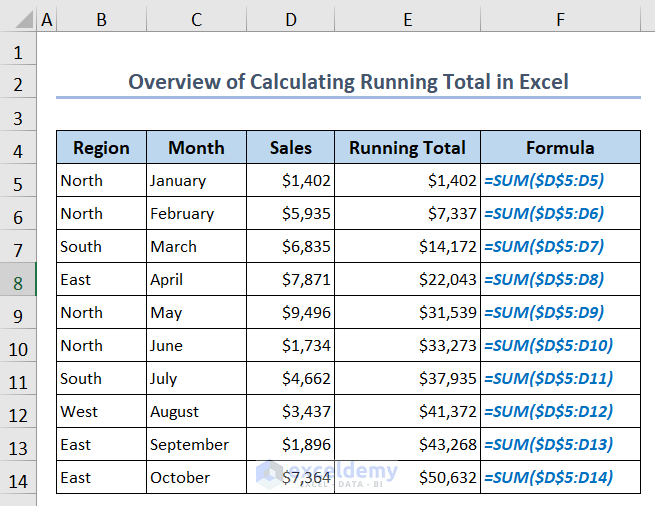
In the following overview image, we used the SUM function to calculate the running total of sales values, with the formulas showing how the function is updated ...

In the following overview image, we selected a range as the source in the Data Validation dialog to create a drop-down list. ⏷Ways of Making ...

Excel is an effective tool for visualizing and analyzing data. Sparklines, a type of small chart in Excel, can be used to represent trends and changes in data ...
See Our Reviews at


Hello,
Thanks for your comment.
There was a small mistake in the formula. That’s why it is giving a Name error. The article and workbook are corrected and updated accordingly. If you have other queries let us know in the comment.
Regards,
Sajid Ahmed
Exceldemy
Hello,
Thanks for your comment.
The formulas are all right. They are working very nicely in our case. You have to insert the formulas carefully in the conditional formatting. Make sure you have put the cell references either absolute or relative correctly. Or if you can provide more information about your dataset then we could help.
If you have other queries let us know in the comment.
Regards,
Sajid Ahmed
Exceldemy
Hello TOM,
Thanks for your comment.
Suppose, you have the following dataset with data in a single column in cells B5:B8. You want to add single quotes and separate them with a comma in cell B11. So, use the following formula with the CONCATENATE function in cell B11:
=CONCATENATE(“‘”,B5,”‘”,”, “,”‘”,B6,”‘”,”, “,”‘”,B7,”‘”,”, “,”‘”,B8,”‘”)
Press Enter to get the desired output.
If you have other queries let me know in the comment.
Regards,
Sajid Ahmed
Exceldemy
Hello DRIN,
Thanks for your comment.
If you want to sum Notebook from India up to France and use drop-down for the countries, then use the following formula in cell C13:
=SUM(INDEX($B$5:$G$8,MATCH(C10,$B$5:$B$8,0),MATCH(C11,$C$4:$G$4,0)+1):INDEX($B$5:$G$8,MATCH(C10,$B$5:$B$8,0),MATCH(C12,$C$4:$G$4,0)+1))
It’ll give the desired result.
Change the countries to China and Germany from the drop-down and the total value will be updated.
If you have other queries let me know in the comment.
Regards,
Sajid Ahmed
Exceldemy
Hello ALEXANDER,
Thanks for your comment.
First, calculate the amortization schedule for the original loan. Then, calculate the amortization schedule for the additional loan separately. Now that you have the monthly payments for both loans, you can combine them to create a single amortization schedule. You’ll need to add the monthly payments together for each month and subtract this total from the outstanding balance.
Repeat this process for each month until both loans are fully paid off. The combined amortization schedule will show the monthly payments and remaining balances as you pay off both loans simultaneously.
If you have other queries let me know in the comment.
Regards,
Sajid Ahmed
Exceldemy
Hlw Jon S M,
Thanks for your comment.
If a customer has more than one invoice with different dates, you have to include multiple rows for that customer in the dataset. Each row will represent a separate invoice entry.
The information related to that customer, such as their name, will be repeated in each row for their respective invoices. But the dates, invoice ids and invoice amounts will be different. The rest of the process is similar with this article.
If you have other queries let me know in the comment.
Regards,
Sajid Ahmed
Exceldemy
Hello Hermione,
Thanks for your comment.
The “Run-time error ‘9’: Subscript out of range” error typically occurs when VBA code tries to reference a worksheet or object that doesn’t exist in the current workbook. In your case, the error is likely occurring because there is no worksheet named “all books” in your Excel workbook.
To fix this issue, you need to ensure that the worksheet name you’re trying to reference (“all books”) exactly matches the name of a worksheet in your workbook. If the worksheet name is different or contains typos or extra spaces, you will encounter this error.
If you have other queries let me know in the comment.
Regards,
Sajid Ahmed
Exceldemy
Hlw Terrisa,
Thank you very much for your comment. The right formula for your need is given below-
=IFERROR(MIN((DATEDIF(W6,TODAY(),”d”)+1)/(DATEDIF(W6,X6,”d”)+1), 1), 0)
Here, we add the MIN function to cap the calculated percentage to 100%. If the calculated percentage is greater than 100%, this function will return 100%, capping the percentage. If the calculated percentage is less than or equal to 100%, it will return the calculated percentage as it is.
If you have other queries let me know in the comment.
Regards,
Sajid Ahmed
Exceldemy
Thank you very much for your valuable comment. You are right. The ASCII character 160 is different than character 32. If you have any cell containing the ASCII character 160 non-breaking space then the TRIM function described in method 1 won’t work.
However, you can use the combination of the SUBSTITUTE and CHAR functions then. Suppose you have a value in cell A1 of your dataset containing the ASCII character 160 non-breaking space. Then you can use the following formula to remove unwanted spaces-
=SUBSTITUTE(A1,CHAR(160), “”)
After using this formula you can apply the Remove Duplicates button.
Regards
Sajid Ahmed
ExcelDemy
Hello Ayodeji Aboderin, thanks for reaching out. You are right, there was an error. Now, the article is updated accordingly. Please let us know if you have any other queries.
Regards
Sajid Ahmed
Exceldemy