How to Do a GST Reconciliation in Excel (4 Methods)

What Is GST Reconciliation in Excel?

GST (Goods and Services Tax) is a tax applied to items you purchase or services you use. It’s added to the cost of goods and services. GST reconciliation in Excel involves comparing and matching data from various sources to ensure the accuracy and completeness of GST-related transactions recorded in a business’s accounting or financial records. The goal is to identify any discrepancies between the GST amounts declared in tax returns and the GST amounts reported in the business’s books.

Dataset Overview

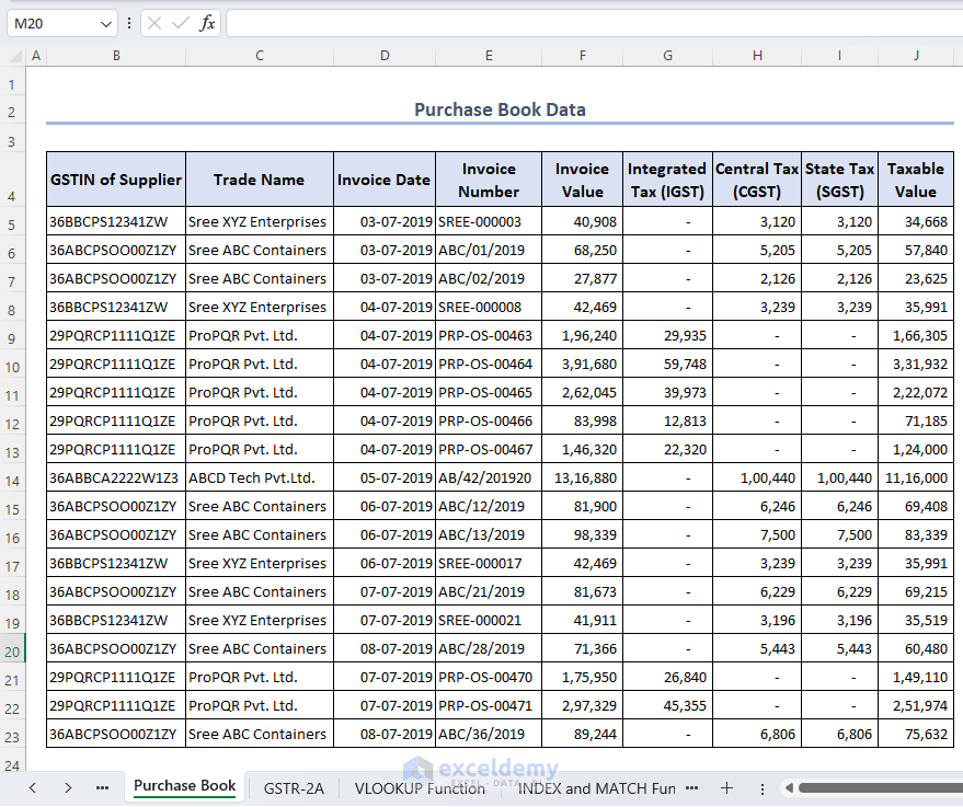
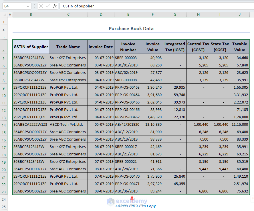
We have two datasets. The first dataset contains purchase book data, including the GSTIN of the supplier, trade name, invoice date, invoice number, invoice value, taxable value, and different types of GST values. Typically, this dataset can be obtained from a company’s accounting records.

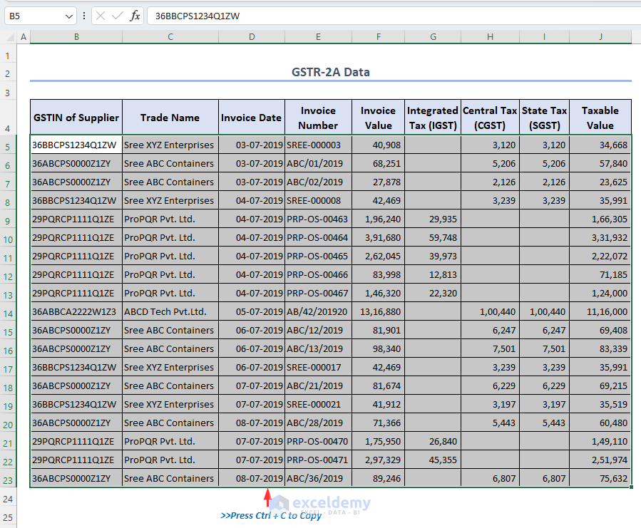
The GSTR-2A data has the same headings as the purchase book data. It provides a comprehensive view of all the inward supplies received during a particular tax period. This dataset is available to registered taxpayers on the GST portal.

We will use these two datasets to perform GST reconciliation in Excel using four suitable methods.

Method 1 – Using the VLOOKUP Function

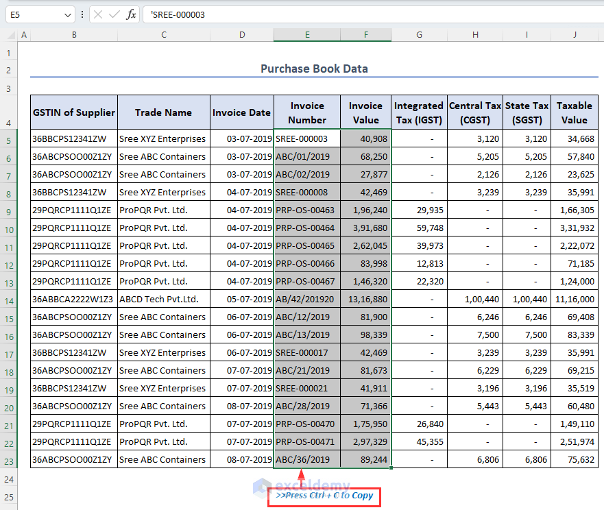
• Copy Invoice Numbers and Invoice Values:
  • Navigate to the purchase book dataset.
  • Copy the invoice numbers and invoice values by pressing Ctrl + C together.

• Create a New Sheet:
  • Open a new sheet in Excel.
  • Select cell B5 and paste the copied values by pressing Ctrl + V together.

• Extract Invoice Values from GSTR-2A:
  • In cell D5, enter the following formula to extract the invoice values from the GSTR-2A dataset based on invoice numbers:

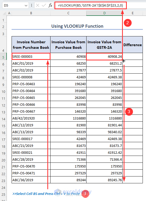
• • Apply the Fill Handle tool to extract the invoice values from the GSTR-2A dataset based on invoice numbers.

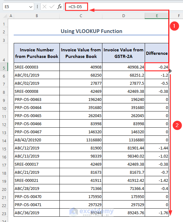
• Calculate the Difference:
  • In cell E5, enter the following formula to calculate the difference in invoice values between the purchase book data and the GSTR-2A data:

• • Apply the Fill Handle tool to obtain the difference in invoice values between the purchase book data and the GSTR-2A data.

• Reconciliation Check:
  • If the difference is 0, the reconciliation is complete.
  • If not, investigate the discrepancies to identify where corrections are needed.

Remember that accurate GST reconciliation ensures compliance and helps maintain precise financial records.

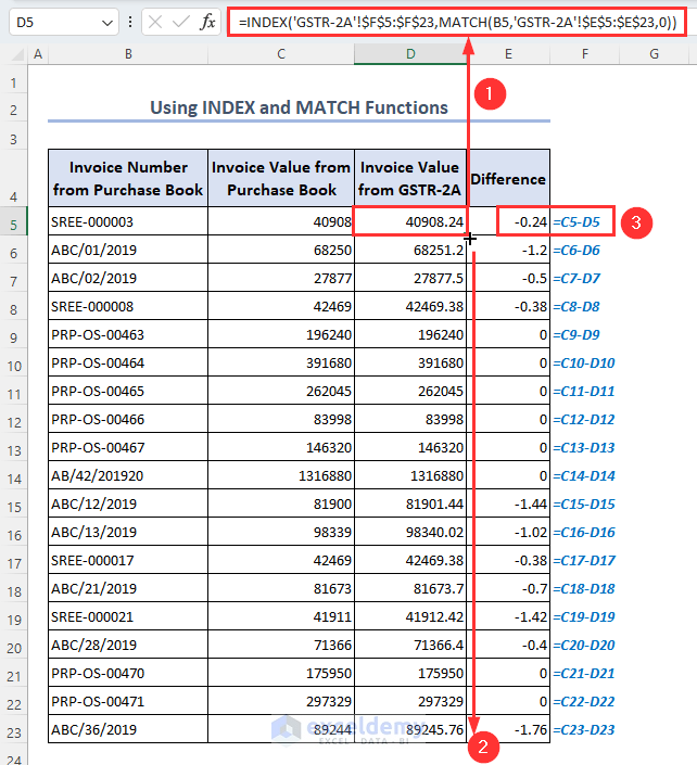
Method 2 – Using the INDEX and MATCH Functions

• Instead of using the VLOOKUP function, you can achieve the same result by combining the INDEX and MATCH functions.
• To extract invoice values from the GSTR-2A dataset based on invoice numbers, follow these steps:
  • In cell D5, enter the following formula:

• Apply the Fill Handle tool to copy this formula down as needed.

• Calculating the Difference in Invoice Values:
  • To find the difference in invoice values between the purchase book data and the GSTR-2A data, enter the formula below in cell E5:

• • Apply the Fill Handle tool to extend this formula as necessary.

Method 3 – Using the SUM Function

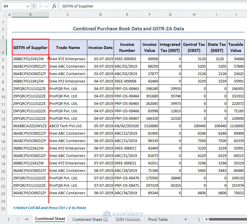
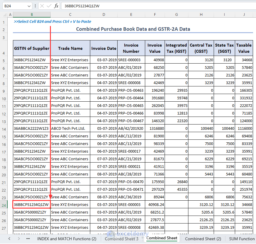
• Combining Datasets:
  • First, combine the two datasets into a single sheet:
    • Copy the entire purchase book dataset (including the header row) by pressing Ctrl + C.

• • • Open a new sheet titled Combined Sheet and select cell B4. Paste the values from the purchase book dataset by pressing Ctrl + V.

• • • Copy the entire GSTR-2A dataset (excluding the header row) by pressing Ctrl + C.

• • • In the Combined Sheet, select cell B24 and paste the GSTR-2A values by pressing Ctrl + V. Now both datasets are in one sheet.

• Calculating GST Reconciliation:
  • Create a new sheet.
  • In cell D5, enter the following formula to get the total integrated tax (IGST), central tax (CGST), state tax (SGST), and taxable values based on the book data:

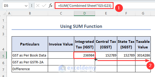
• • • Apply the Fill Handle tool to extend this formula as needed.

• • In cell D6, enter the following formula to get the total GST values from the GSTR-2A data:

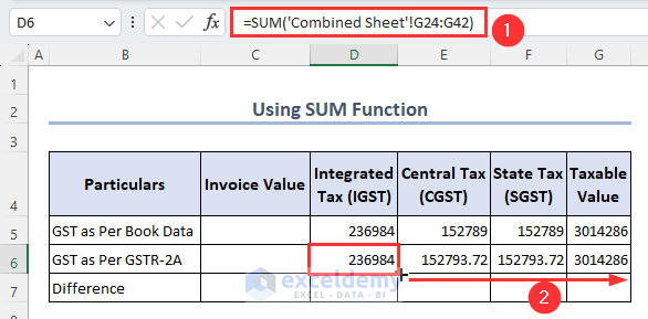
• • • Use the Fill Handle tool to copy this formula down.

• • To calculate the total GST values as invoice values, enter the following formula in cell C5:

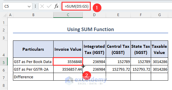
• • • Apply the Fill Handle tool to fill down as necessary.

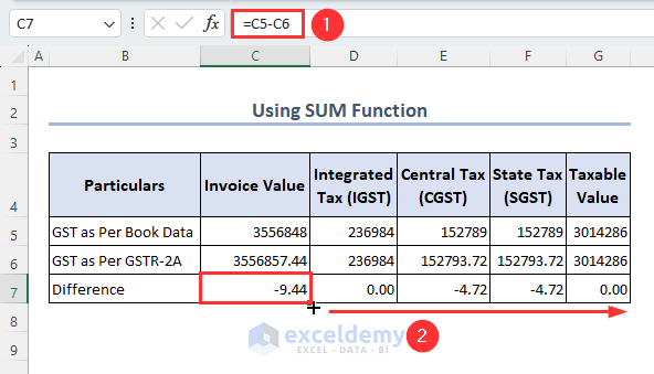
• • Find the differences between the datasets by typing the following formula in cell C7:

• • Use the Fill Handle tool to copy this formula down.
  • The reconciliation process is now complete.

Method 4 – Using the Pivot Table

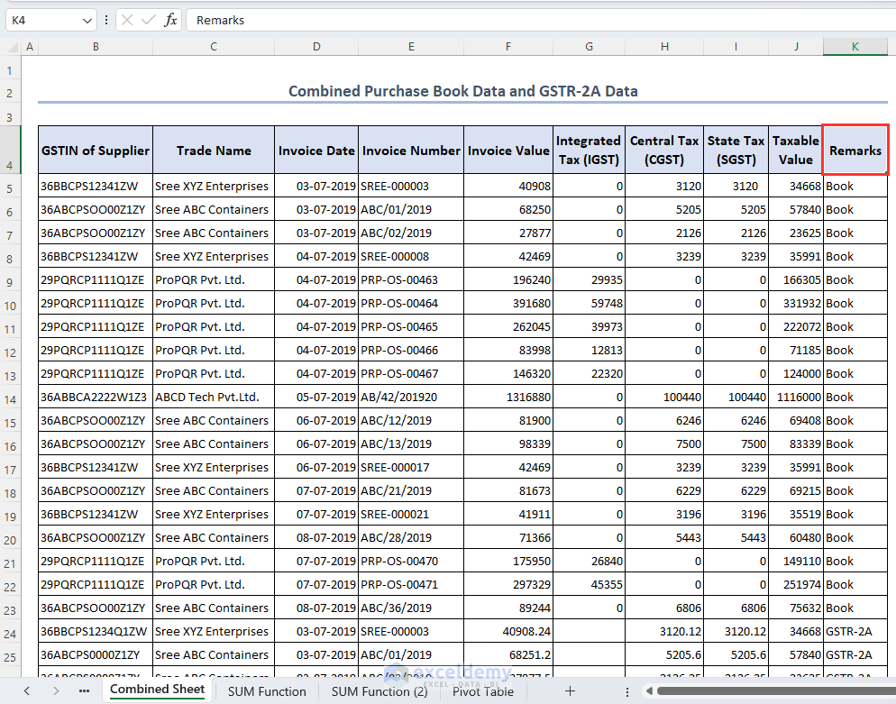
• Creating a New Column for Remarks:
  • Open the Combined Sheet.
  • Insert a new column titled Remarks.
  • In this column, label the rows corresponding to the purchase book data as Book and the rows corresponding to the GSTR-2A data as “GSTR-2A.” This will help identify the source of the data.

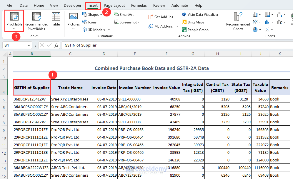
• Setting Up the Pivot Table:
  • Select any cell (for example, cell B4) in the Combined Sheet.
  • Go to the Insert tab and choose PivotTable.

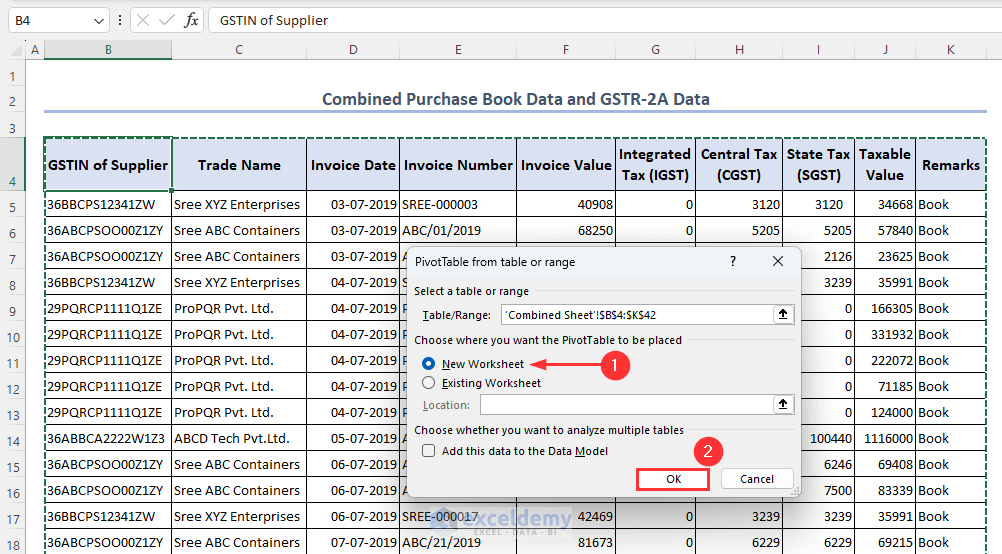
• Creating the Pivot Table:
  • Choose New Worksheet as the position for the Pivot Table and click OK.
  • The Pivot Table will now display summarized data based on the selected fields.

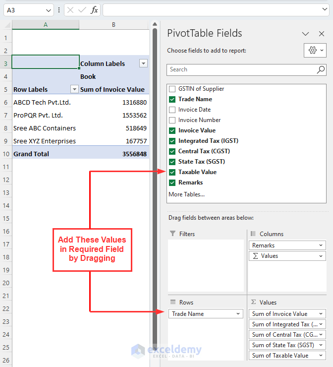
• • In the PivotTable Fields window, select the necessary fields:
    • Drag Trade Name to the Rows field.
    • Drag Remarks to the Columns field.
    • Also, drag Invoice Value, Integrated Tax (IGST), Central Tax (CGST), State Tax (SGST), and Taxable Value to the Values field.

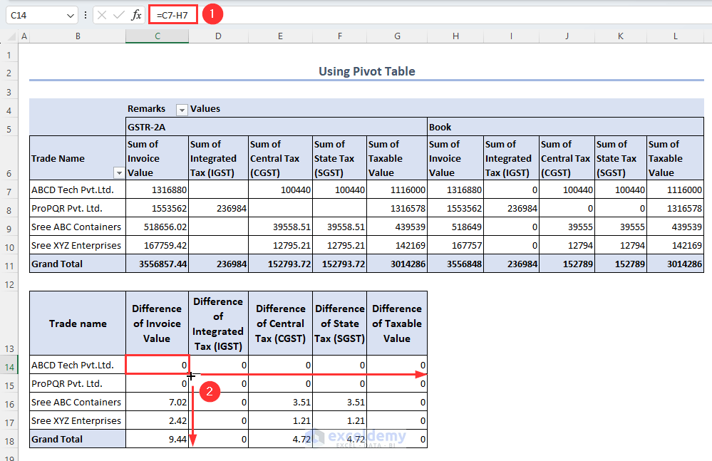
• Calculating the Difference:
  • In cell C14, enter the following formula:

• • • Apply the Fill Handle tool in either direction to obtain the difference between the GST and total values from the purchase book data and the GSTR-2A data.

The reconciliation process is now complete using the Pivot Table.

Download Practice Workbook

You can download the practice workbook from here:

Frequently Asked Questions (FAQs)

• What precautions should I take during GST reconciliation in Excel?
  • Always maintain backups of your original data.
  • Ensure that your Excel formulas are accurate.
  • Double-check your calculations and reconciliations.
  • Document the reconciliation process for auditing purposes.

• How often should I perform GST reconciliation in Excel?
  • It is recommended to perform GST reconciliation monthly. Regular reconciliation helps identify discrepancies early and ensures accurate reporting.