How to Reconcile Data in 2 Excel Sheets: 4 Ways

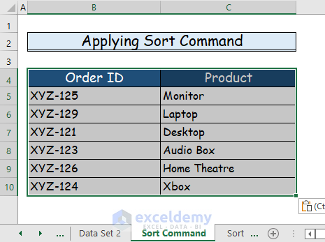
Method 1 – Applying Sort Command to Reconcile Data in 2 Excel Sheets

Step 1:

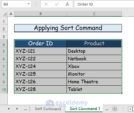
• Select the data range of cell B4:C10 from the first worksheet.

Step 2:

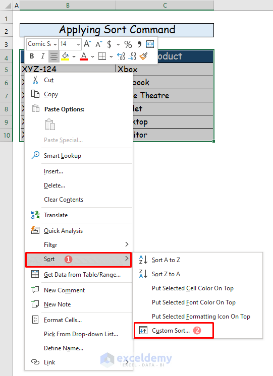
• Right-click on the data range and select the Sort command.
• From the sort options, choose the Custom Sort… command.

Step 3:

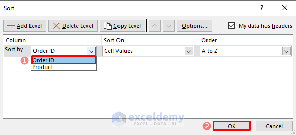
• See the Sort dialogue box.
• In the Sort by dialogue box, select Order ID.
• Press OK.

Step 4:

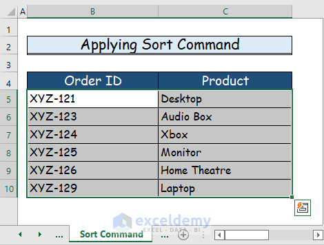
• See the first data set will be sorted in terms of Order ID.

Step 5:

• Apply the Sort command to sort the second data set as well.

Step 6:

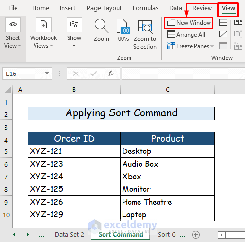
• Create a side-by-side view for both worksheets.
• Go to the View tab of the ribbon.
• In the Window group, select the New Window command.

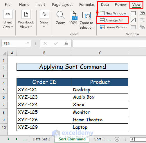
Step 7:

• From the View tab, choose the Arrange All command.

Step 8:

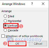
• See the Arrange Windows window.
• Under the Arrange heading, select Vertical.
• Press OK.

Step 9:

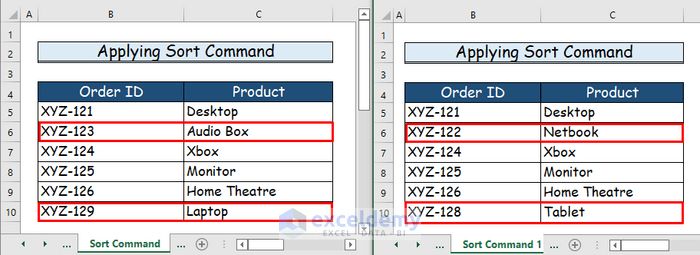
• See the two worksheets side-by-side after this action.
• Identify any similarities or dissimilarities between them after carefully going through the data sets.

Method 2 – Using COUNTIF Function to Reconcile Data in 2 Excel Sheets

Step 1:

• Select the side-by-side view for the worksheets as shown in the previous method.
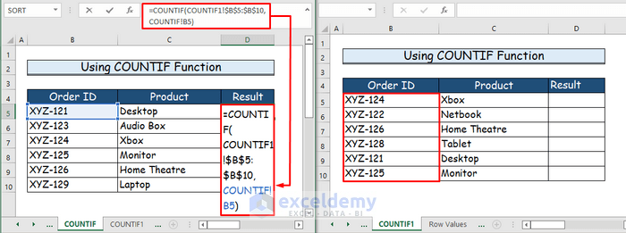
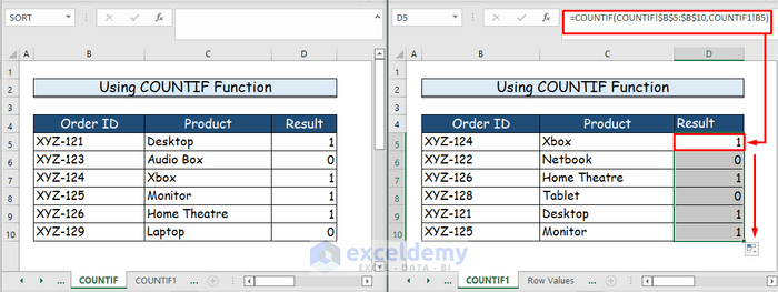
• In cell B5 of our first worksheet, type the following formula for the COUNTIF function.

• We are selecting the data range from cell B5:B10 of the second worksheet for comparison.

Step 2:

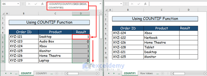
• Press Enter to get the result.
• Use the AutoFill feature to drag the formula to the lower cells.
• You will get 1 or 0 as a result.
• 1 indicates if the first data set has any matching value with the second one.
• 0 indicates no match of data.

Step 3:

• Apply the following formula of the COUNTIF function in cell B5 of the second data set.

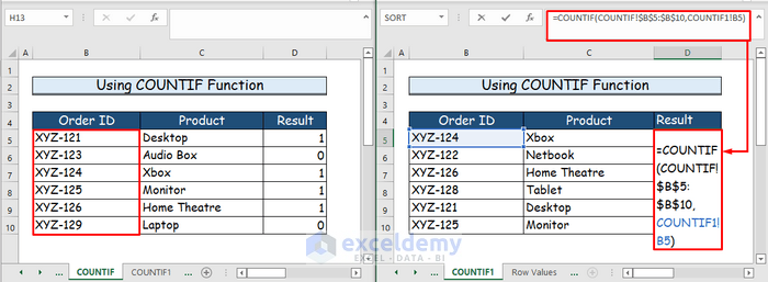
Step 4:

• Press Enter to see the result.
• Use the AutoFill feature to get the results of the lower cells.

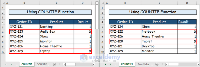
Step 5:

• See the similarities or dissimilarities between the data sets automatically in the form of 1 or 0.

Method 3 – Matching Row Values to Reconcile Data in 2 Excel Sheets

Step 1:

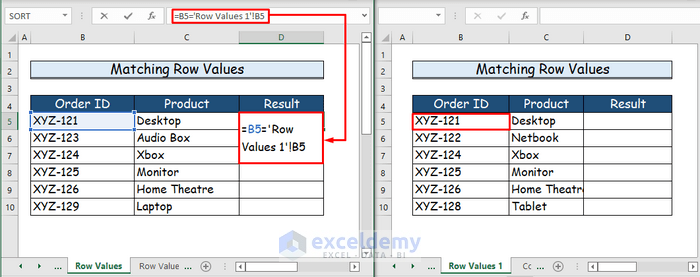
• To compare row values type the following formula in cell B5 of the first data set.

• Match each row value of the first and second data sheets.

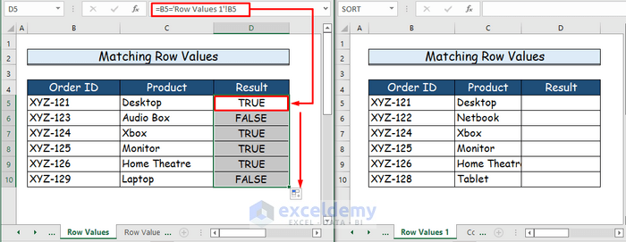
Step 2:

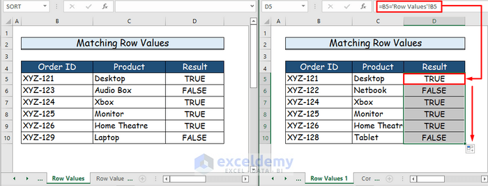
• Press Enter and drag the formula to the lower cells using AutoFill.
• If any of the row values match with the same row values of the second data set it will show TRUE as a result.
• It will show False.

Step 3:

• In cell B5 of the second data set, write the following formula.

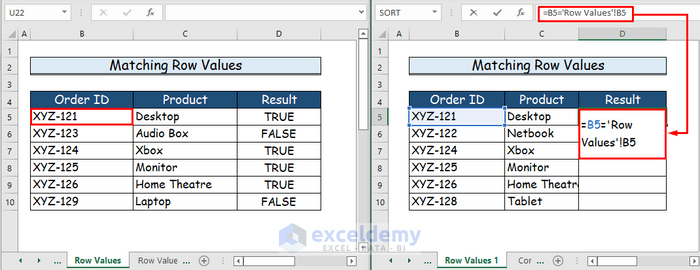
Step 4:

• Press Enter and drag the formula to the lower cells using AutoFill.

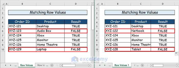
Step 5:

• Compare or match the row values of the two data sets by following the above steps.

Method 4 – Utilizing Conditional Formatting to Reconcile Data

Step 1:

• Set the side-by-side view for both worksheets.

Step 2:

• In the first worksheet, select the data range B5:C10.
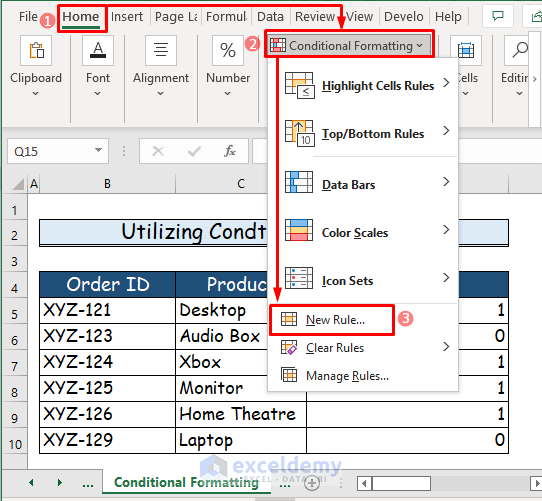
• From the Home tab, select Conditional Formatting.
• From the drop-down, select the New Rule option.

Step 3:

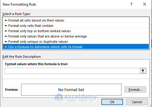
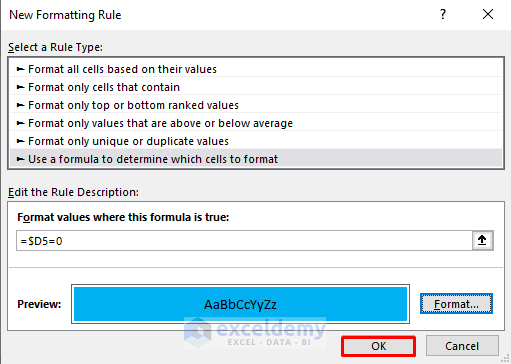
• See the New Formatting Rule dialogue box.
• Go to the Select a Rule Type heading.
• Select the option named “Use a formula to determine which cells to format”.

Step 4:

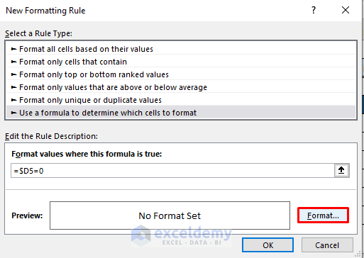
• Type the following formula in the Edit the Rule Description box.

• Choose the Format command.

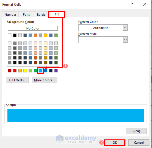
Step 5:

• From the Fill tab of the Format Cells dialogue box, choose any color of your preference.
• Press OK.

Step 6:

• The dialogue box from Step 4 will be back with all the editing.
• Press OK.

Step 7:

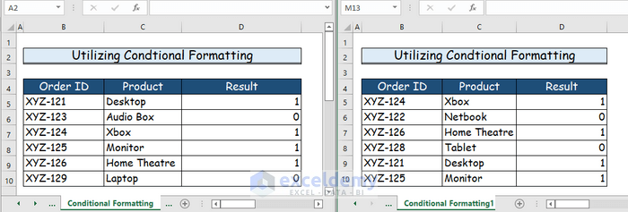
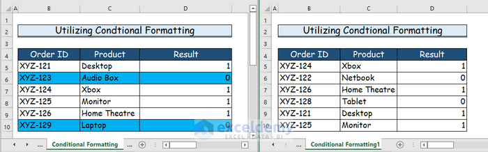
• Your first data set will look like the following picture after completing all the steps.
• After formatting, the cells with 0 in them will be highlighted, meaning they do not match.

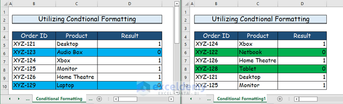
Step 8:

• Repeat Step 1 to Step 6 to get the result for the second data set as well.

Download Practice Workbook

You can download the free Excel workbook here and practice on your own.

Related Articles

• How to Do Bank Reconciliation in Excel
• How to Do Intercompany Reconciliation in Excel
• Automation of Bank Reconciliation with Excel Macros
• How to Perform Bank Reconciliation Using VLOOKUP in Excel
• How to Reconcile Credit Card Statements in Excel

<< Go Back to Excel Reconciliation Formula | Excel for Accounting | Learn Excel