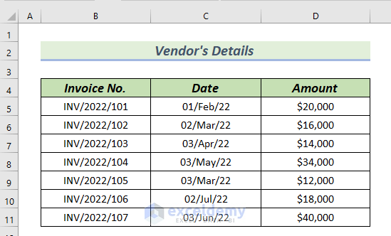
The following Vendor’s Details table has Invoice No., Date, and Amount columns. The Amount column shows the vendor’s demand for a particular invoice.
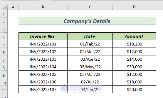
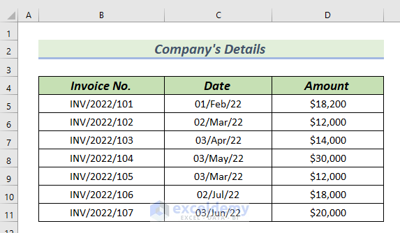
The following Company’s Details table shows Invoice No., Date and Amount columns. The Amount column shows what the vendor has gained from the company for a particular invoice.
There is a difference between what the vendor has demanded and what the vendor has gained from the company. Therefore, the vendor statement needs reconciliation.
Method 1 – Using Pivot Table to Reconcile Vendor Statement in Excel
Step 1 – Making Dataset
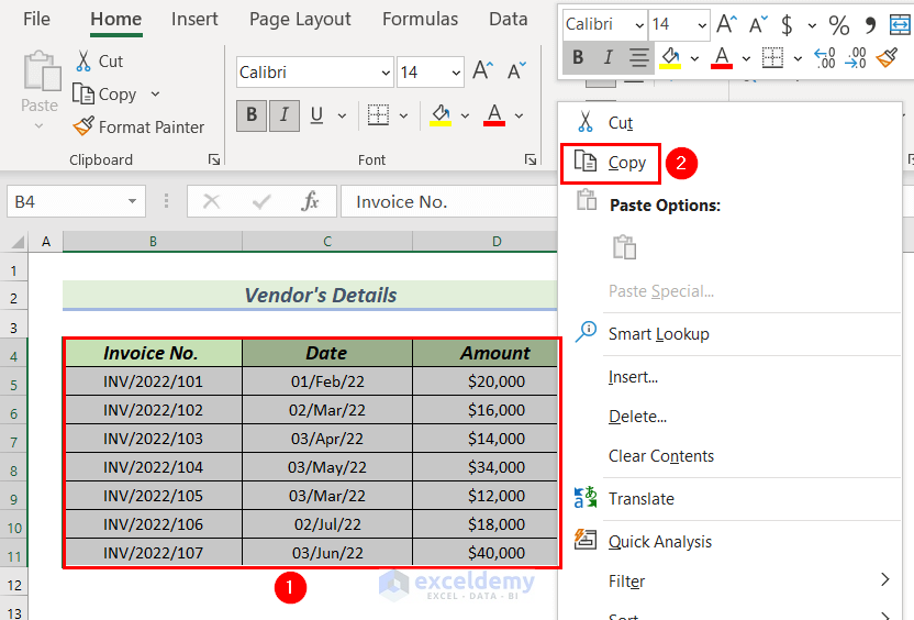
- Select the entire dataset of the Vendor’s Details (You can select the entire dataset by clicking on cell B4 and pressing CTRL+SHIFT+END).
- Right-click and select Copy from the Context Menu. (You can copy the dataset by pressing CTRL+C).
- Paste the copied cell into another worksheet.
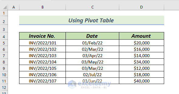
- Click on cell B4and press CTRL+V.
This shows the Vendor’s Details as shown in the image below.
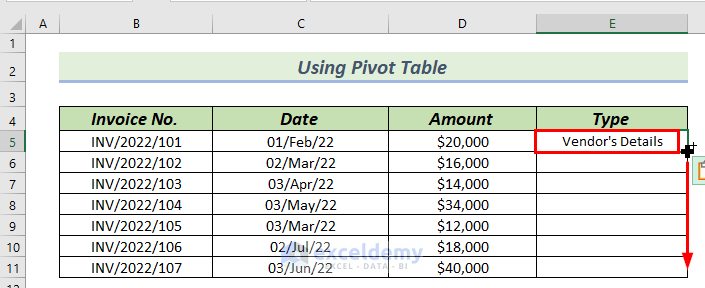
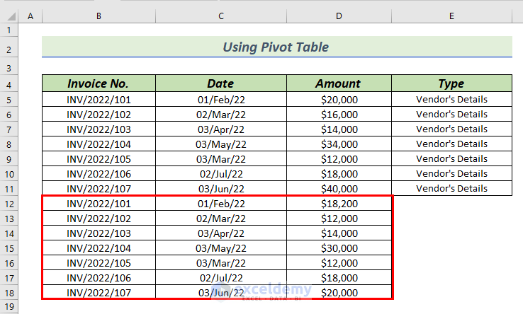
Add a Type column in the dataset.
- Add Vendor’s Details in cell E5.
- Drag down the cell content of cell E5 with the Fill Handle tool.
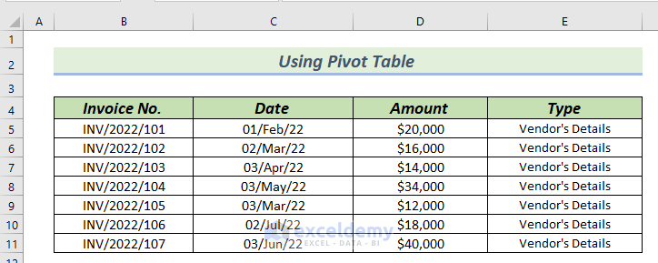
This shows the Vendor’s Details as shown in the image below.
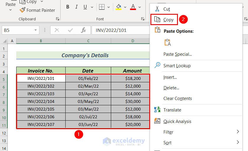
To add the Company’s Details to the same dataset.
- Copy the data from the Company’s Details
- Exclude the heading.
- Select cells B5:D11>> right-click on it.
- Select Copy from the Context Menu.
Go back to the dataset to insert Pivot Table.
- Click on cell B12 and paste.
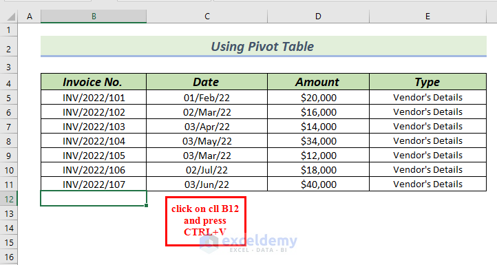
This shows the Company’s Details data in the dataset.
To add the Company’s Details in the Type column.
- Type Company’s Details in cell E12.
- Drag down the cell content of cell E12 with the Fill Handle tool.
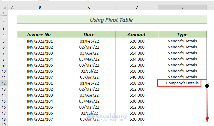
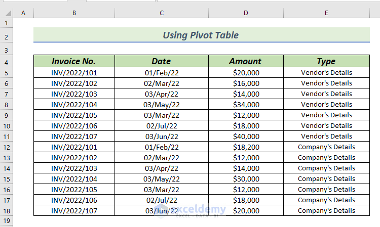
This shows the complete dataset.
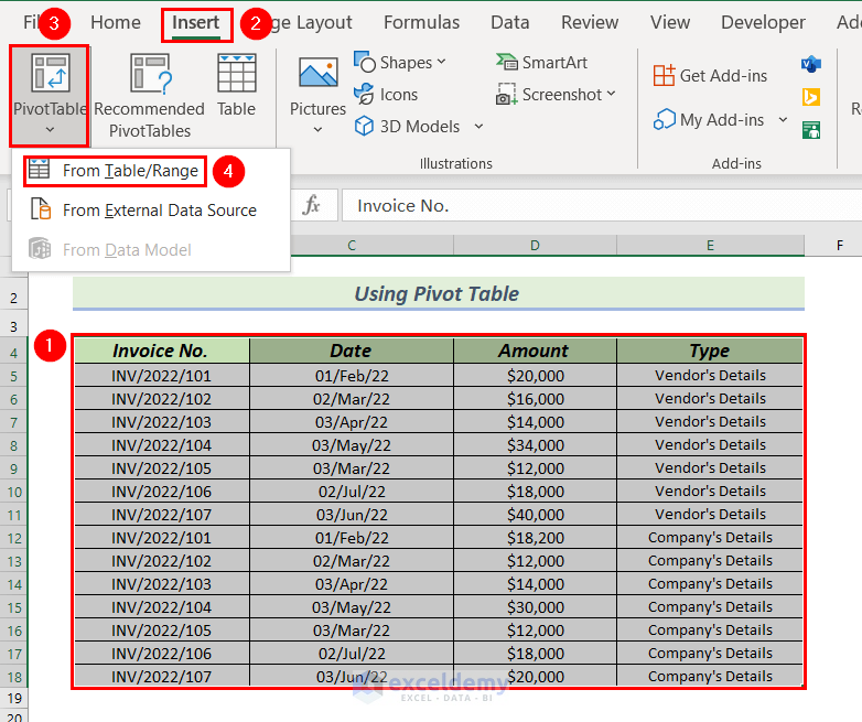
Step 2 – Inserting Pivot Table
- Select the entire dataset >> go to the Insert
- From Pivot Table group >> select From Table/Range.
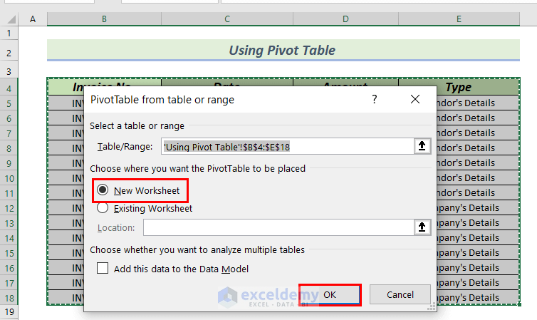
A PivotTable from table or range dialog box will pop up.
Mark the New Worksheet.
- Click OK.
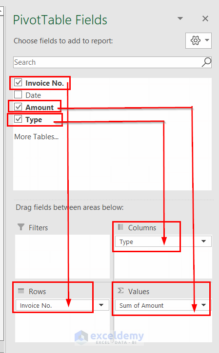
The PivotTable Fields is now in a new worksheet.
- Check the Invoice No. and drag it down to the Rows
- Check the Amount and drag it down to the Values
- Check theType and drag it down to the Columns
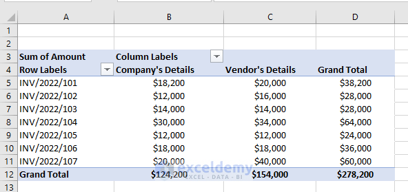
The Pivot Table is created.
To remove the Grand Total column from the Pivot Table.
- Select the Grand Total column >> go to the Design
- From Grand Totals>> select Off Rows and Columns.
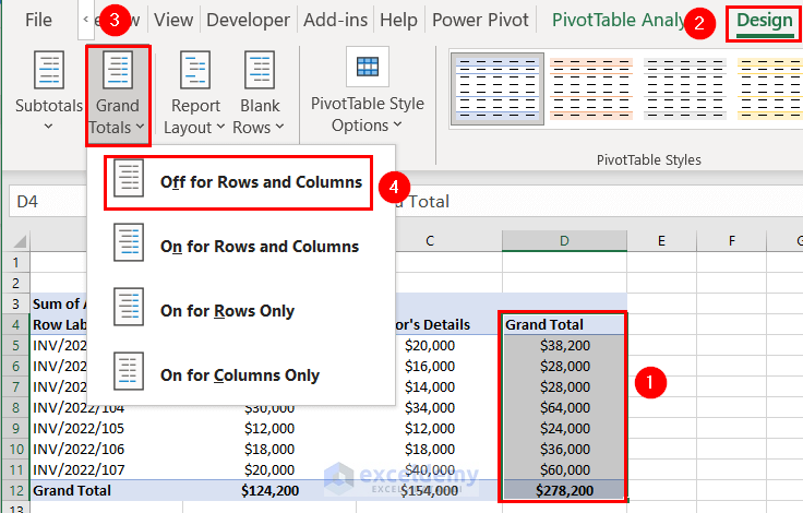
The Grand Total column is removed.
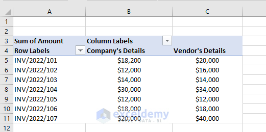
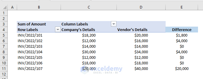
To find the difference between Company’s Details and the Vendor’s Details, add a heading named Difference in the Pivot Table.
- Insert following formula in cell D5.
=D5-C5This finds out the difference between vendor demand and vendor gain.
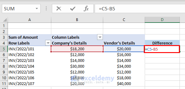
- Press ENTER.
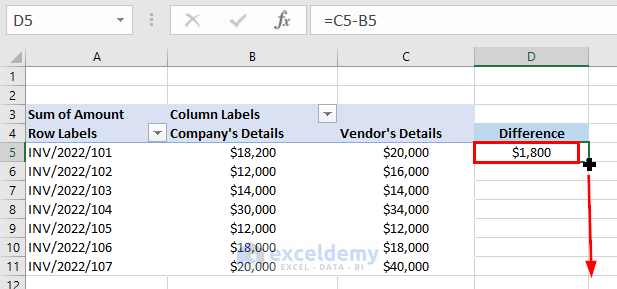
- You can see the result in cell D5.
- Drag down the formula with the Fill Handle tool.
The complete Difference column is now shown.
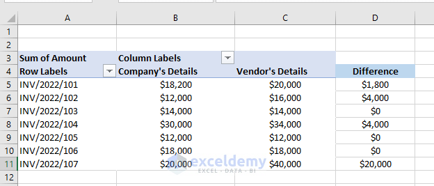
- To make the Pivot Table more presentable remove the gridlines from the worksheet and inserted a column at A.
- The reconciliation vendor statement is now complete.
Read More: How to Do Intercompany Reconciliation in Excel
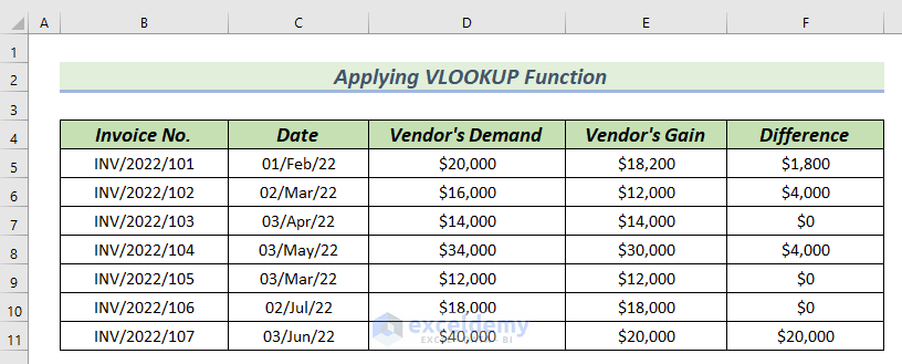
Method 2 – Applying VLOOKUP Function to Reconcile Vendor Statement in Excel
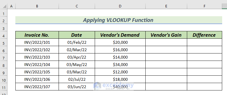
The following dataset has Invoice No., Date and Vendor’s Demand columns with an incomplete Vendor’s Gain and Difference column.
The VLOOKUP function needs a table_array to look up a value. Use Company’s Detail table as the table_array.
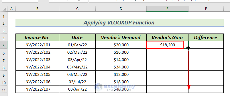
- Insert the following formula in cell E5.
=VLOOKUP(B5,'Company''s Detail'!$B$4:$D$11,3,FALSE)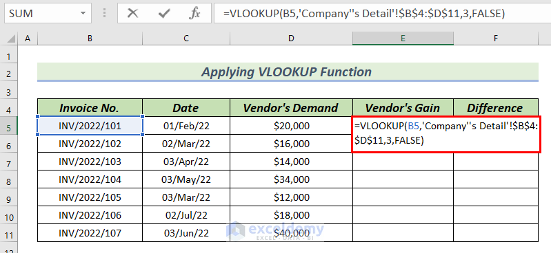
Formula Breakdown
- VLOOKUP(B5,’Company”s Detail’!$B$4:$D$11,3,FALSE) → the VLOOKUP function looks for values in a fixed column index of a table array.
- B5 → is the lookup_value.
- ‘Company”s Detail’!$B$4:$D$11 → is the table_array.
- 3 → is the column_index_number.
- FALSE → indicates the Exact match.
- Output: $18200
- Explanation: $18200 is the Vendor’s Gain for Invoice No. INV/2022/101.
- Press ENTER to get the result in cell E5.
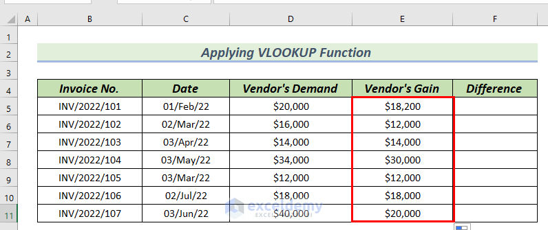
- Drag down the formula with the Fill Handle tool.
You can see the complete Vendor’s Gain column.
- Insert the following formula in cell F5.
=D5-E5This subtracts Vendor’s Gain from Vendor’s Demand.
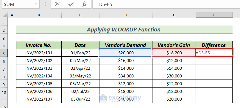
- Press ENTER to get the result in cell F5.
- Drag down the formula with the Fill Handle tool.
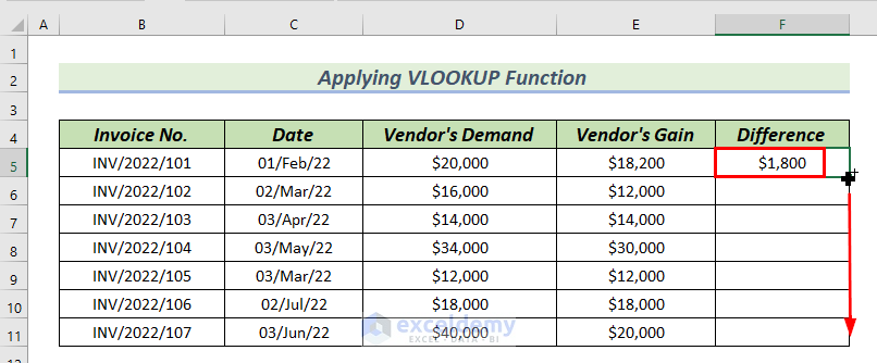
You can see the complete Difference column.
Read More: How to Perform Bank Reconciliation Using VLOOKUP in Excel
Download Practice Workbook
Related Articles
- How to Do Bank Reconciliation in Excel
- Automation of Bank Reconciliation with Excel Macros
- How to Reconcile Two Sets of Data in Excel
- How to Reconcile Data in Excel
- How to Reconcile Data in 2 Excel Sheets
- How to Reconcile Credit Card Statements in Excel
<< Go Back to Excel Reconciliation Formula | Excel for Accounting | Learn Excel
Get FREE Advanced Excel Exercises with Solutions!
