This is an overview.
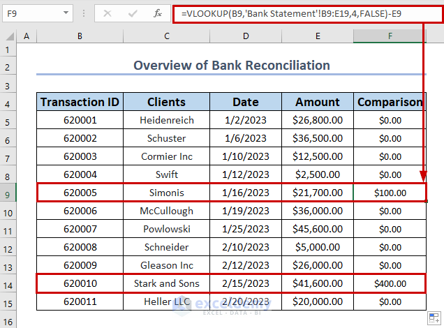
There are transaction rows with discrepancies.
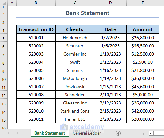
Step 1 – Create a Dataset
The first dataset is a Bank Statement: Transaction ID is the unique identification number of each transaction, Clients shows the name of the organization, Date has date information, and Amount holds the transaction amount.
The second dataset is General Ledger. It is an accountant record.
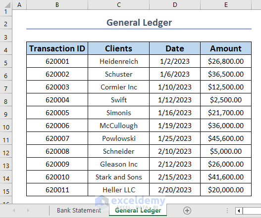
Match the General Ledger dataset with the Bank Statement dataset to reconcile the amount:
Read More: Automation of Bank Reconciliation with Excel Macros
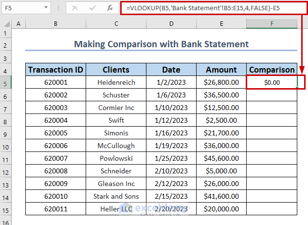
Step 2 – Calculate Differences Using the VLOOKUP Function
Insert a column in the General Ledger dataset.
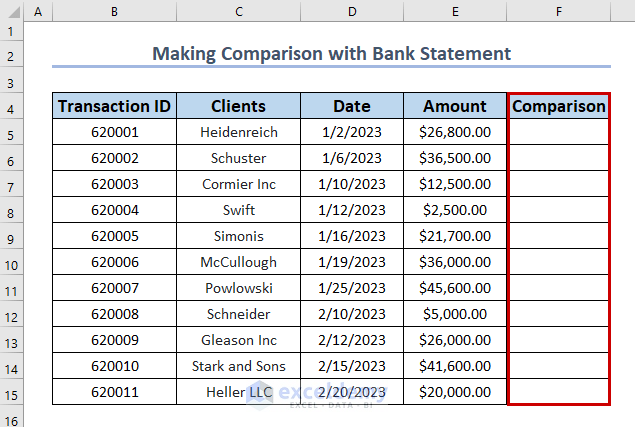
Compare the Amount columns:
Find exact matches with the VLOOKUP function, and subtract the Amount of General Ledger from the Amount of the Bank Statement.
- Select F5.
- Enter the following formula:
=VLOOKUP(B5,'Bank Statement'!B5:E15,4, FALSE)-E5
Formula Breakdown
- VLOOKUP(B5,’Bank Statement’!B5:E15,4, FALSE) → The VLOOKUP function searches for the exact match of Transaction ID betweeen both datasets and return the value.
- B5 is the lookup value: the Transaction ID of General Ledger.
- ‘Bank Statement’!B5:E15 is the lookup array: the whole dataset of Bank Statement.
- 4 is the column number of Amount.
- FALSE is the condition for an exact match.
- Output → $26,800.00.
- VLOOKUP(B5,’Bank Statement’!B5:E15,4,FALSE)-E5 → becomes
- $26,800.00-E5 → the Amount of both datasets is subtracted.
- Output → $0.00.
- $26,800.00-E5 → the Amount of both datasets is subtracted.
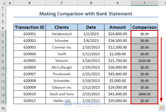
- Drag down the Fill Handle to see the result in the rest of the cells.
Read More: How to Reconcile Two Sets of Data in Excel
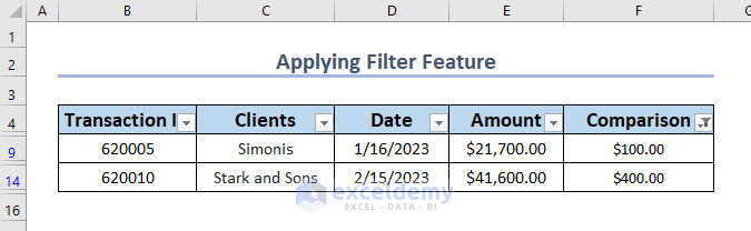
Step 3 – Applying the Filter Feature to Highlight Transactions With Discrepancies
Filter cells with values of $0.00.
- Select the whole dataset.
- Select Filter in Sort & Filter in the Editing group.
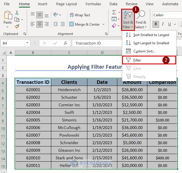
- Click Filter.
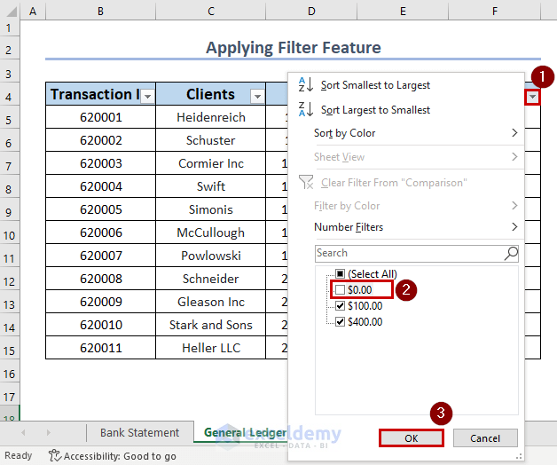
- Uncheck $0.00.
General Ledger displays the Amount of discrepancies only.
This is the output.
Read More: How to Reconcile Data in Excel
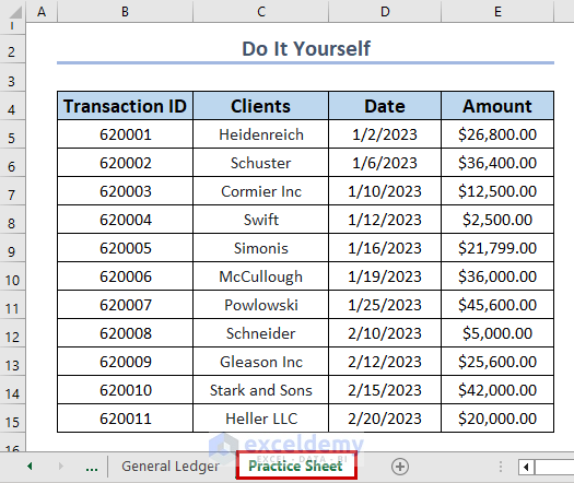
Practice Section
Practice here.
Download Practice Workbook
Download the practice workbook.
Related Articles
- How to Do Reconciliation in Excel
- How to Do Bank Reconciliation in Excel
- How to Reconcile Data in 2 Excel Sheets
- How to Do Intercompany Reconciliation in Excel
- How to Reconcile Vendor Statements in Excel
- How to Reconcile Credit Card Statements in Excel
<< Go Back to Excel Reconciliation Formula | Excel for Accounting | Learn Excel
Get FREE Advanced Excel Exercises with Solutions!
