In this article, we will demonstrate how to use the VLOOKUP, INDEX, MATCH and SUMIF functions to perform data reconciliation in Excel.
Download Practice Workbook
What Is Reconciliation?
The word reconciliation means the restoration of friendly relationships, and data reconciliation refers to the process of data verification, matching and comparing figures for accuracy.
We discover dissimilarities between multiple sets of data by performing data reconciliation, which can be performed at regular time intervals or during the sharing of data.
Reconciliation in Excel: 4 Formulas
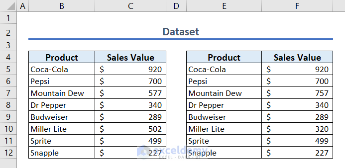
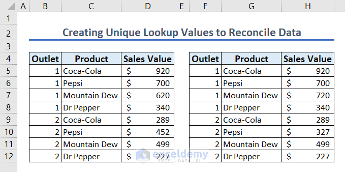
Our sample dataset has two segments. The left segment (B4:C12) is from the central database, whereas the right (E5:F12) is from the current worksheet. Let’s reconcile these two datasets.
Method 1 – Using VLOOKUP Function
Steps:
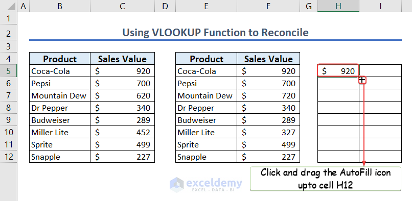
- Enter the following formula in cell H5 and press ENTER:
=VLOOKUP(E5,$B$5:$C$12,2,FALSE)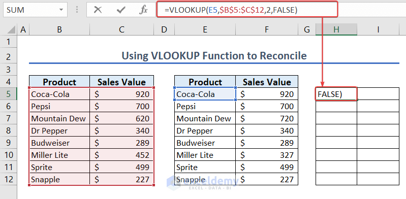
The sales value of Coca-Cola from the central dataset (B4:C12) is returned.
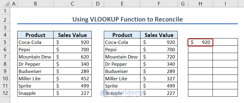
Yo get the values for all the other products, we’ll use the AutoFill feature.
- Select cell H5 and place the cursor around the bottom right corner.
- As the AutoFill icon shows up, click and drag it down to cell H12.
We have all the products’ sales values.
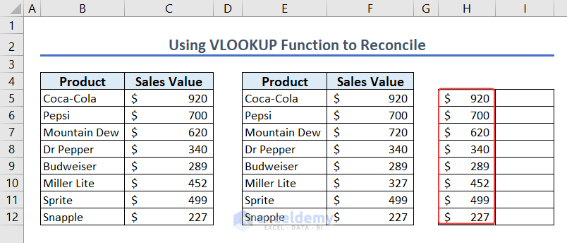
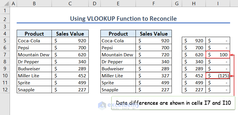
Now, we calculate the difference between the sales values in the central and current databases.
- Enter the following formula in cell I5 and press ENTER:
=F5-H5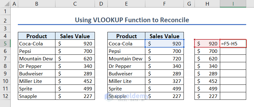
As a result, we have the difference for the product Coca-Cola. We can see a ‘–’ symbol as the difference is zero (0).
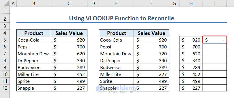
- Use the AutoFill feature to get the difference for all the other products.
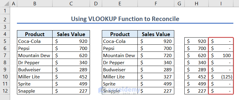
From the reconciliation, we can say there are variances for the Mountain Dew and Miller Lite products.

Method 2 – Using INDEX and MATCH Functions
Steps:
- Enter the following formula in cell H5 and press ENTER:
=INDEX($C$5:$C$12,MATCH(E5,$B$5:$B$12,0))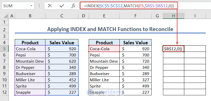
We have the sales value of Coca-Cola from the central dataset (B4:C12).
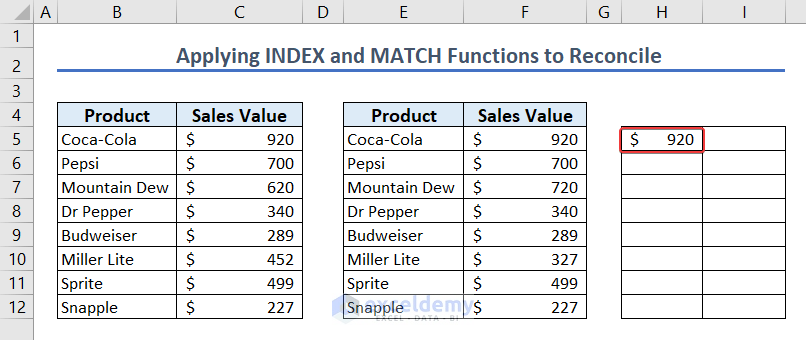
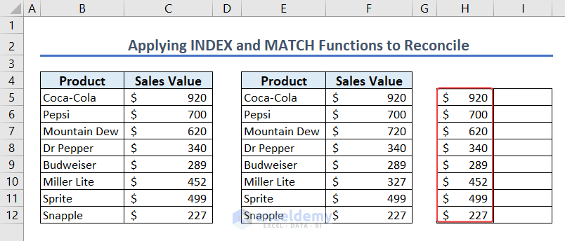
- Use the AutoFill feature to get the sales values for all the other products.
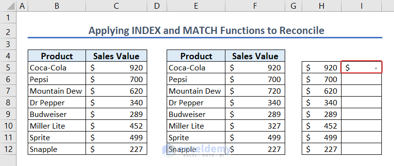
- Enter the following formula in cell I5 and press ENTER:
=F5-H5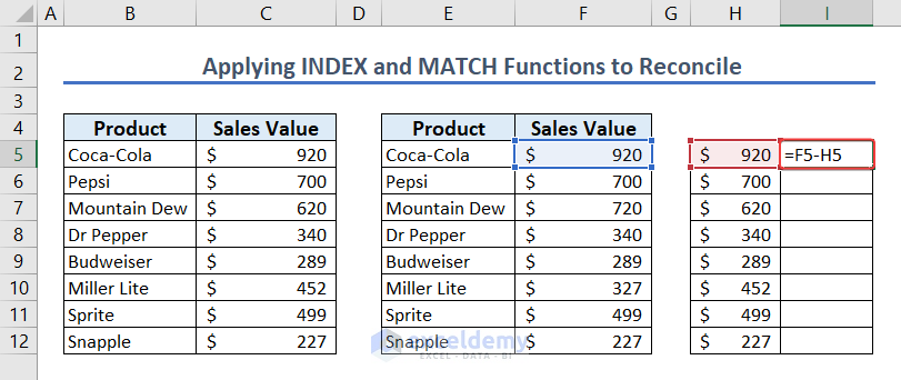
We have the difference between the central and the current datasets for Coca-Cola.
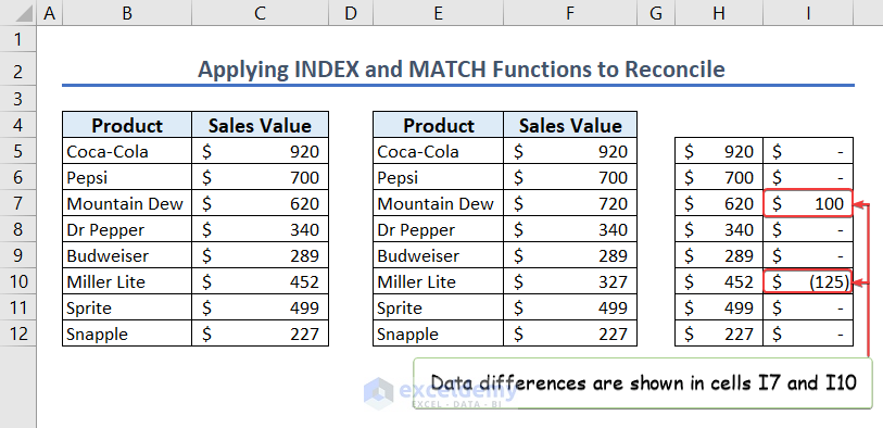
- Use the AutoFill feature to get the corresponding values for all the other products.
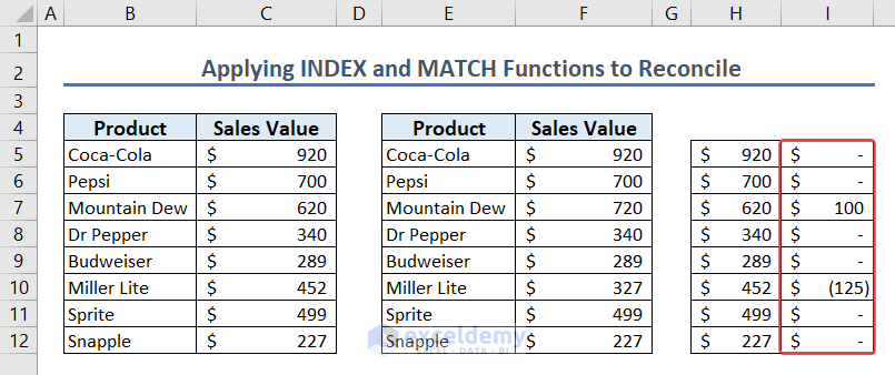
We can see from the following image that there are variances in cells I7 and I10.
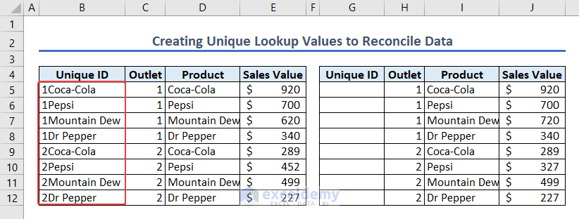
Method 3 – Creating Unique Lookup Values to Reconcile Data
If there is repetition in our dataset, the VLOOKUP function returns the result based on the first match it finds.
This produces an inconsistent result.
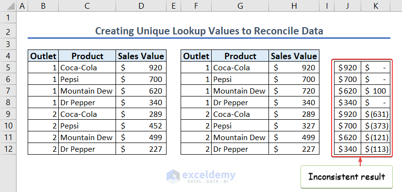
We can create a unique id to overcome this issue.
Steps:
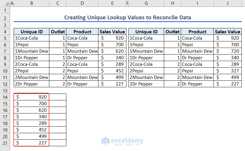
- Enter the following formula in cell B5 and press ENTER:
=C5&D5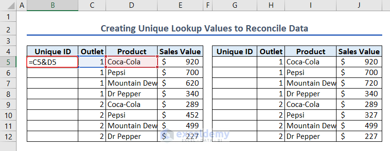
We have the outlet number and product name combined as a unique id.
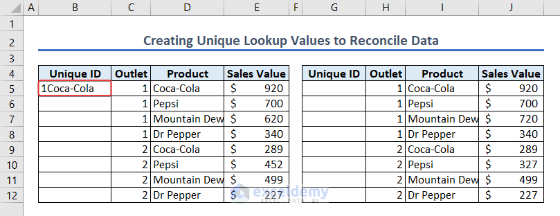
- Use the AutoFill feature to repeat the process for all the other products.
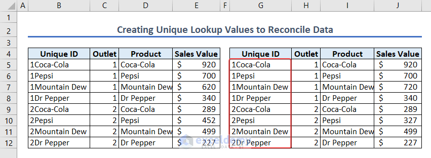
- Similarly, create the unique id for the current dataset too.
- Enter the following formula in cell B14 and hit ENTER:
=VLOOKUP(G5,$B$5:$E$12,4,FALSE)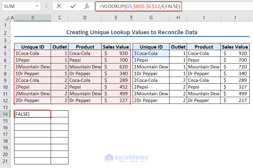
We have the sales value for Coca-Cola using our unique id.
- Use the AutoFill feature to get the sales values for all the other products.
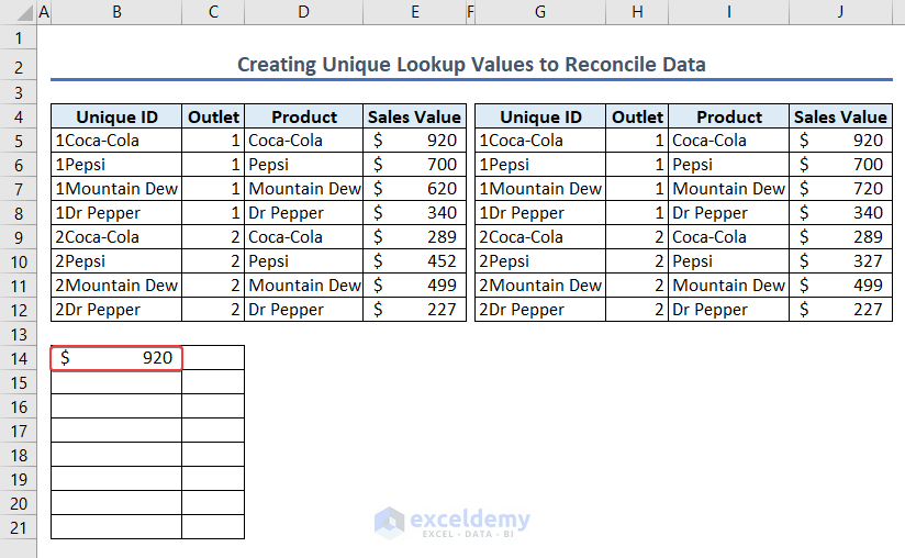
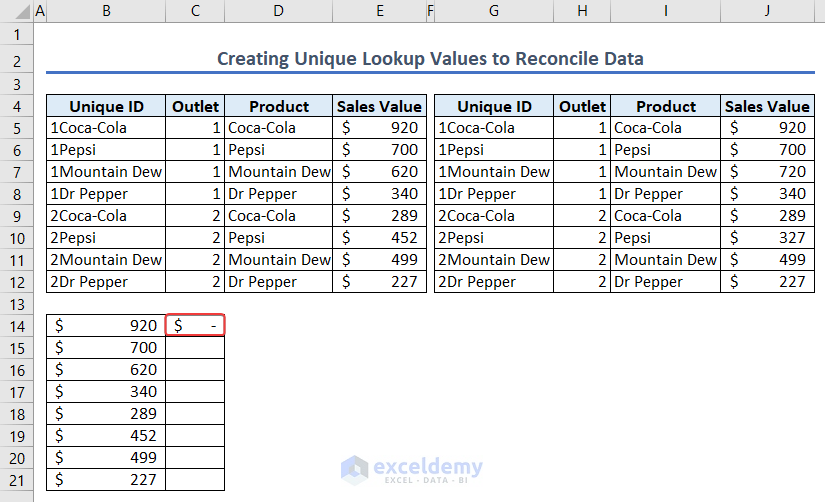
- Enter the following formula in cell C14 and press ENTER:
=J5-B14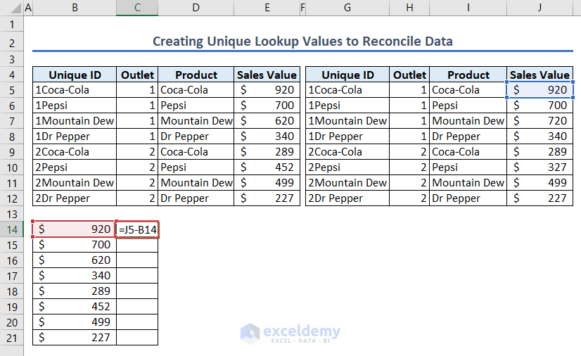
As the difference is zero (0), we get ‘–’ as output.
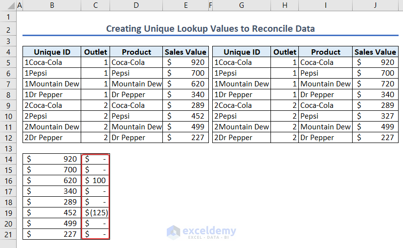
- Use the AutoFill feature to get the difference for all the other products.
The following image shows variances in cells C16 and C19, which refer to 1Mountain Dew and 2Pepsi.
Method 4 – Using Combination of ROUND And SUMIF Functions
In this case, we are provided data about four customers in cells G4:H8, and will use the ROUND and SUMIF functions to create a reconciliation formula in Excel.
We need to verify the data in cells B4:D14.
Steps:
- Enter the following formula in cell E5 and hit ENTER:
=SUMIF($B$5:$B$14,"="&B5,$D$5:$D$14)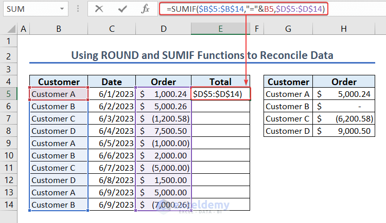
We have the Total Order amount for Customer A in cell E4.
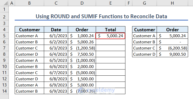
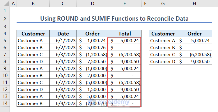
- Use the AutoFill feature to get the values for all the other customers.
The data is verified in terms of Total Order.
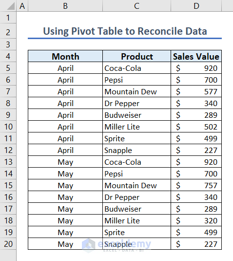
How to Create a Pivot Table to Reconcile Data
Our dataset looks like this.
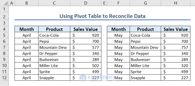
We need to create a merged dataset first.
Steps:
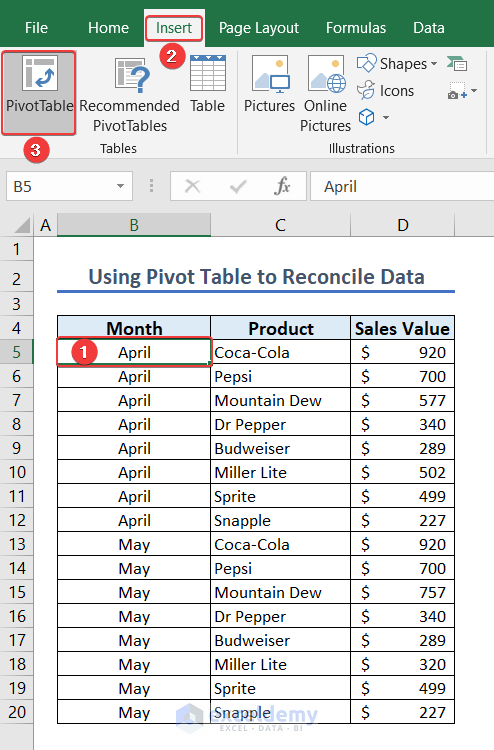
- Select any cell in the dataset (cell B5 in this case), and go to Insert >> PivotTable.
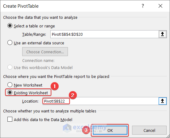
A Create PivotTable window will pop up.
- Select the options as shown in the following image and click OK.
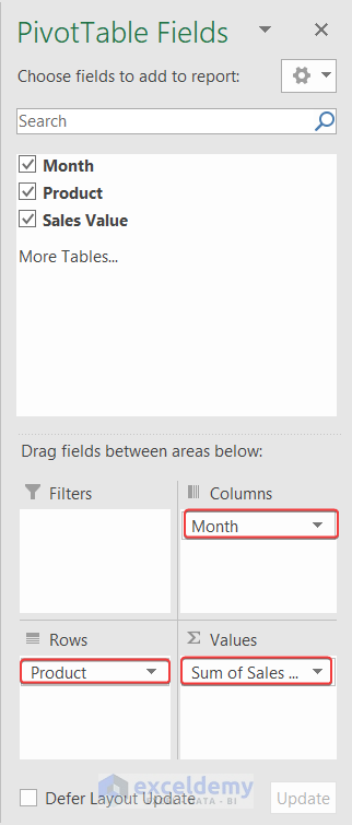
The PivotTable Fields window will appear on the right side of the active worksheet.
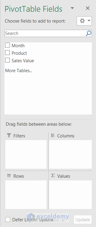
- Drag and drop the fields into the respective PivotTable fields as shown in the following image.
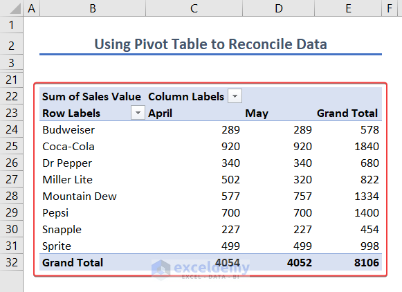
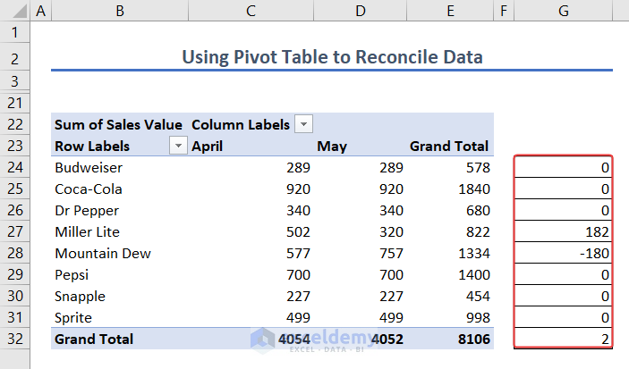
We have a pivot table like the following image.
- Enter the following formula in cell G24 and press ENTER:
=C24-D24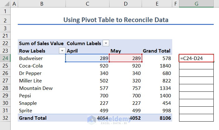
We have the difference between April and May.
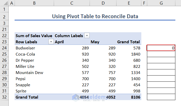
- Use the AutoFill feature to get the values for all the other products.
Data reconciliation has been performed.
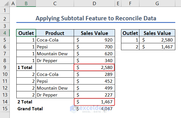
Reconciliation of Data Using Subtotal Feature
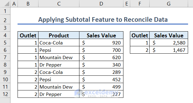
We can also use the Subtotal feature to reconcile data. In the dataset below, the sales values for outlets 1 and 2 are provided in cells F4:G6.
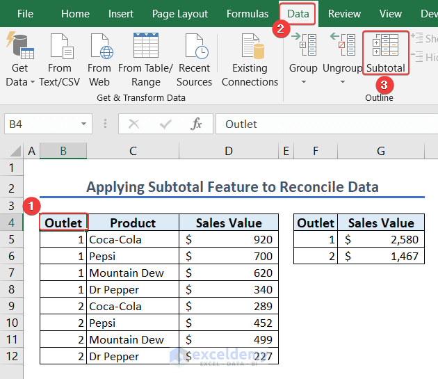
- Select any cell from the worksheet (cell B4 in this case), and go to Data >> Subtotal to create a subtotal.
A Subtotal window will pop up.
- Select the options as shown in the following image and click OK.
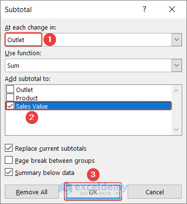
We have the total sales value of outlets 1 and 2.
- Cross-check it with the values of cells G5 & G6.
The values match.
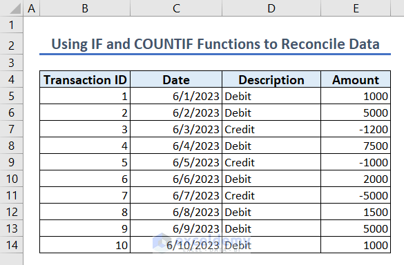
How to Perform Reconciliation in a Bank
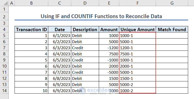
We can use the IF and COUNTIF functions to accomplish this. The dataset looks like the following image. Note that credits are denoted with the minus sign (-). There are repetitive amounts of debit and credit. We’ll label them as “Matched” to distinguish them.
Steps:
- Enter the following formula in cell F5 and press ENTER:
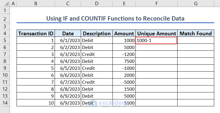
=IF(E5<0,-E5&"-"&COUNTIF(E$5:E5,E5),E5&"-"&COUNTIF(E$5:E5,E5))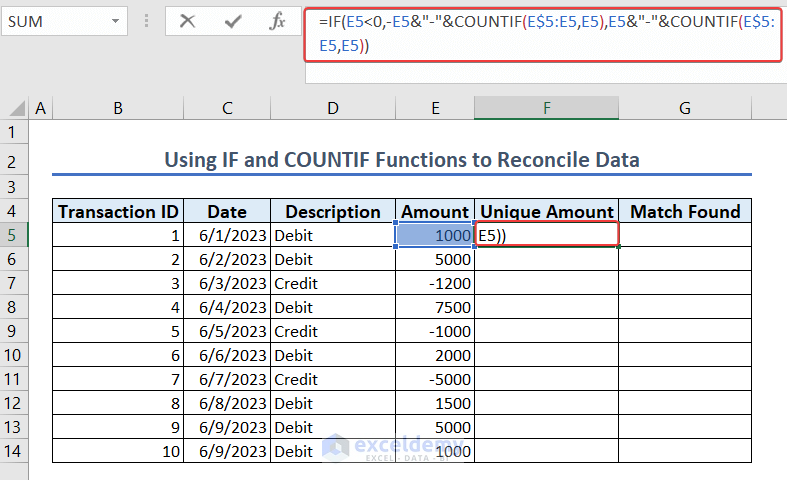
We get a unique amount.
- Use the AutoFill feature to get the values for all the other transactions.
- Enter the following formula in cell G5 and hit ENTER:
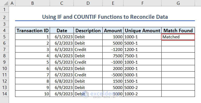
=IF(COUNTIF($F$5:$F$14,F5)=2,"Matched","")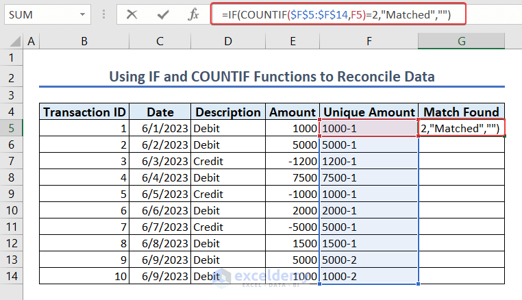
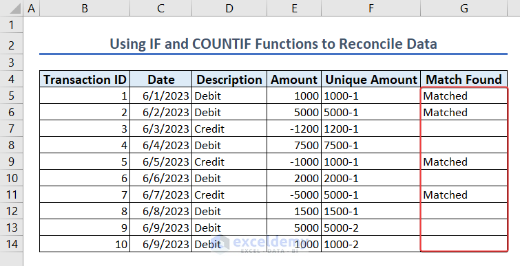
We have the match status.
- Use the AutoFill feature to get the match status for all the other transactions.
Things to Remember
- Enter a formula if you’re referring to data from a pivot table. We cannot select cells from the pivot table as this will enable the GETPIVOTDATA function.
- Create a unique id whenever needed.
- Set the match type as FALSE in the VLOOKUP function, as we need an exact match.
Frequently Asked Questions
1. What is the formula for reconciliation?
A reconciliation formula’s main task is to find the similarities and dissimilarities between two datasets. We can use the VLOOKUP, INDEX, MATCH, and SUMIF functions to reconcile data using formulas. See above for demonstrations.
2. What is data reconciliation in Excel?
Data reconciliation in Excel means comparing two Excel datasets to find similarities and dissimilarities.
3. How to use a formula in Excel?
Select a cell, type =, and start your required formula.
Excel Reconciliation Formula: Knowledge Hub
- Reconciliation in Excel
- Reconcile Data
- Reconcile Two Sets of Data
- Reconcile Data in 2 Excel Sheets
- Bank Reconciliation in Excel
- Bank Reconciliation Using VLOOKUP
- Automation of Bank Reconciliation
- How to Reconcile Credit Card Statements in Excel
- Reconcile Vendor Statements
- Intercompany Reconciliation
<< Go Back to Excel for Accounting | Learn Excel
Get FREE Advanced Excel Exercises with Solutions!
