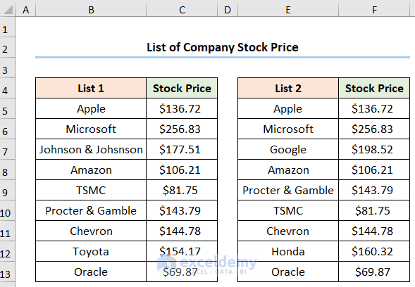
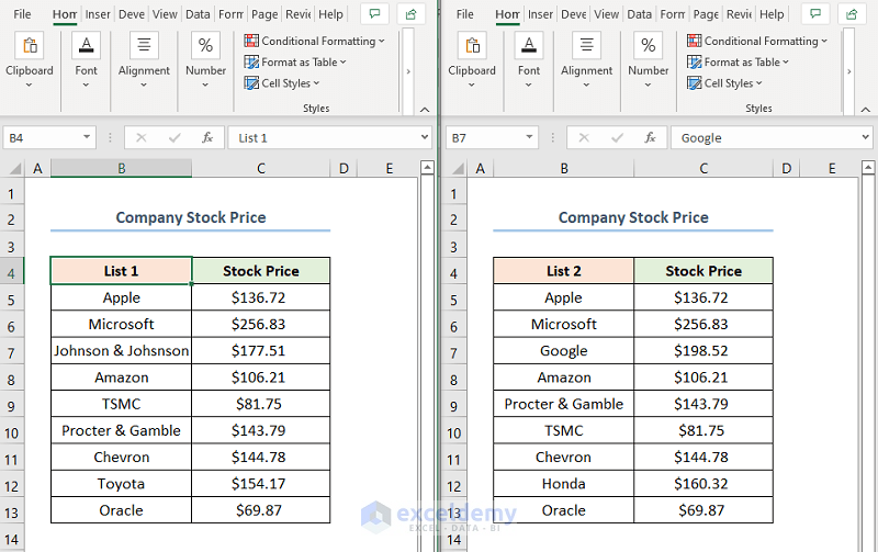
The dataset shows two lists containing Company names and their Stock Prices in USD. We want to check if the two lists are an exact match or if there are any mismatches. To do this, we’ll utilize various Excel tools and functions.
Method 1 – Comparing Rows to Reconcile Two Sets of Data
Steps:
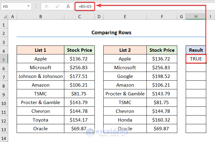
- Insert a column with the header ‘Result’.
- Go to cell H5 and enter the following formula:
=B5=E5
Here, B5 and E5 refer to the value Apple in Lists 1 and 2. When the values of B5 and E5 are the same, it returns TRUE; otherwise, it returns FALSE.
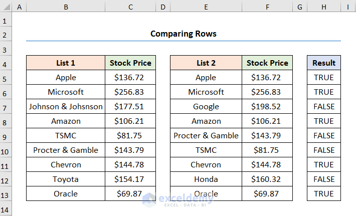
- Use the Fill Handle tool to copy the formula into the cells below.
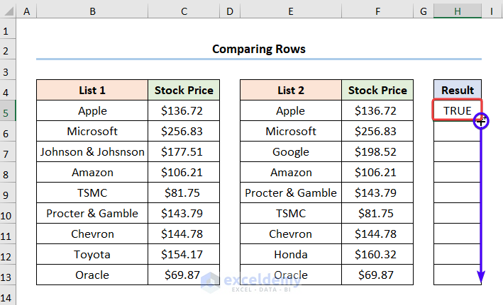
See the results in the image below.
Read More: How to Reconcile Data in 2 Excel Sheets
Method 2: Applying Conditional Formatting to Reconcile Two Sets of Data
Steps:
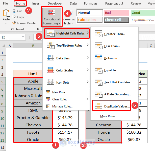
- Select the List 1 and List 2 columns >> in the Home tab, click the Conditional Formatting drop-down >> select the Highlight Cells Rules option >> from the list, and press the Duplicate Values option.
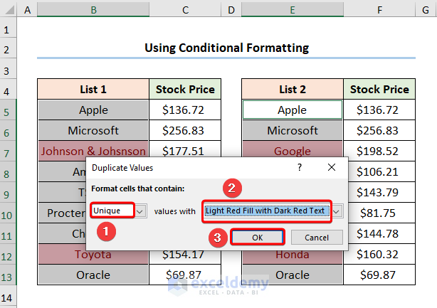
This opens the Duplicate Values wizard.
- Choose the Unique values option >> select Light Red Fill with Dark Red Text as the cell and text colors >> click the OK button.
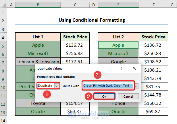
- Choose the Duplicate values option >> select Green Fill with Dark Green Text for the cell and text colors.
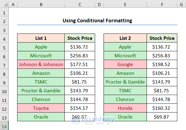
The results should look like the picture given below.
Read More: How to Do Reconciliation in Excel
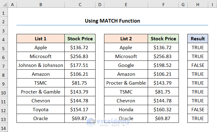
Method 3 – Utilizing the MATCH Function
Steps:
- Go to cell H5 and insert the following formula:
=ISNUMBER(MATCH(E5,$B$5:$B$13,0))
In this formula, cell E5 points to the value Apple while the B5:B13 range represents the List 1 array.
⚡ Formula Breakdown:
- MATCH(E5,$B$5:$B$13,0) → returns the relative position of an item in an array matching the given value. Here, E5 is the lookup_value argument, which refers to Apple. Following, $B$5:$B$13 represents the lookup_array argument from where the value is matched. Lately, 0 is the optional match_type argument, which indicates the Exact match criteria.
- Output → 1
- ISNUMBER(MATCH(E5,$B$5:$B$13,0)) → becomes
- ISNUMBER(1) → the ISNUMBER function checks whether a value is a number and returns TRUE or FALSE. Here, 1 is the value argument, and since it is a number so the function returns TRUE.
- Output → TRUE
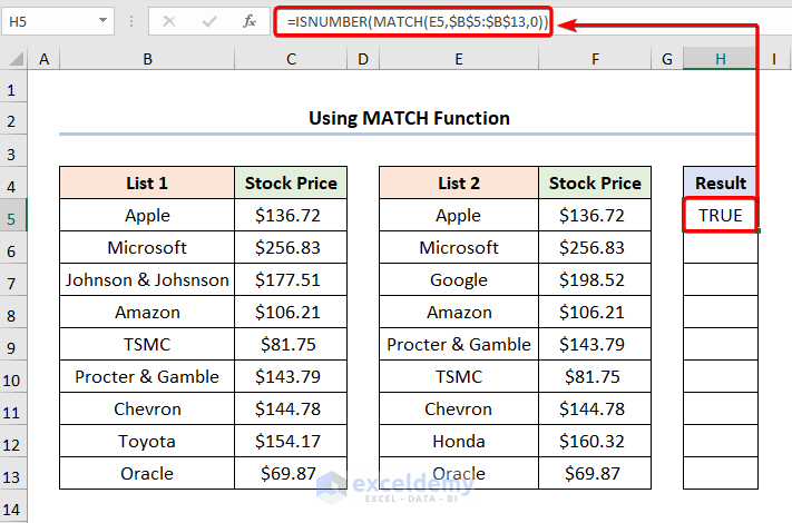
The results should look like the screenshot given below.
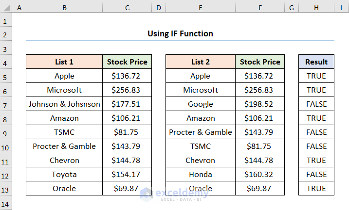
Method 4 – Using the IF Function to Reconcile Two Sets of Data
Steps:
- Go to cell H5 and type in the following formula:
=IF(B5=E5,"TRUE","FALSE")
In the above formula, the B5 and E5 represent the value Apple in List 1 and List 2.
⚡ Formula Breakdown:
- IF(B5=E5,”TRUE”,”FALSE”) → checks whether a condition is met and returns one value if TRUE and another value if FALSE. Here, B5=E5 is the logical_test argument, which checks if the value in the B5 cell equals the E5 cell. If they are equal, the function returns text TRUE (value_if_true argument); otherwise, it returns FALSE (value_if_false argument).
- Output → TRUE
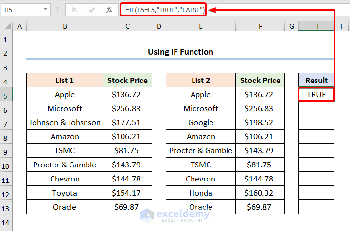
The output should look like the screenshot shown below.
Method 5: Employing the Table Option with the XMATCH Function to Reconcile Two Sets of Data
Steps:
- Select the B4:B13 range of cells >> move to the Insert tab >> click the Table option.
- The Create Table wizard appears where you must check the My table has headers option.
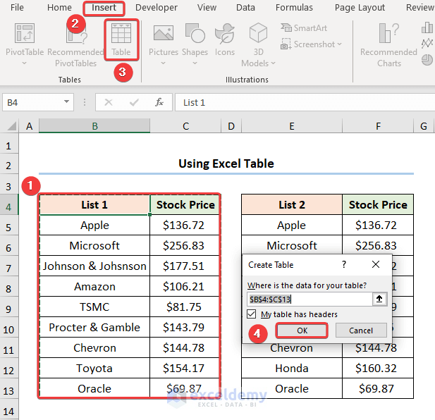
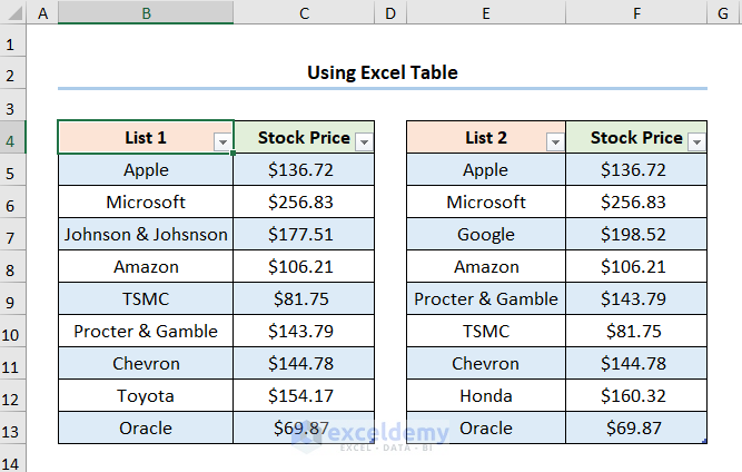
The Table should look like the screenshot below.
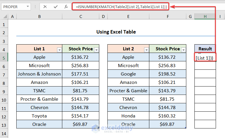
- Go to cell H5 and enter the formula below:
=ISNUMBER(XMATCH(Table2[List 2],Table1[List 1]))
⚡ Formula Breakdown:
- XMATCH(Table [List 2], Table [List 1]) → The XMATCH function returns the relative position of an item in an array by default, requiring an exact match. Here, Table 2 [List 2] is the lookup_value argument, which refers to the B5:B13 array. Table 1 [List 1] represents the lookup_array argument from where the value is matched.
- ISNUMBER(XMATCH(Table2[List 2], Table1[List 1])) → checks whether a value is a number and returns TRUE or FALSE. Here, XMATCH(Table [List 2], Table [List 1]) (value argument) returns an array.
- Output → TRUE
Note: The XMATCH function is available in Excel 365. If you’re using an older version, then you can use the expression below to get the same results.
=ISNUMBER(MATCH(Table2[List 2],Table1[List 1],0))
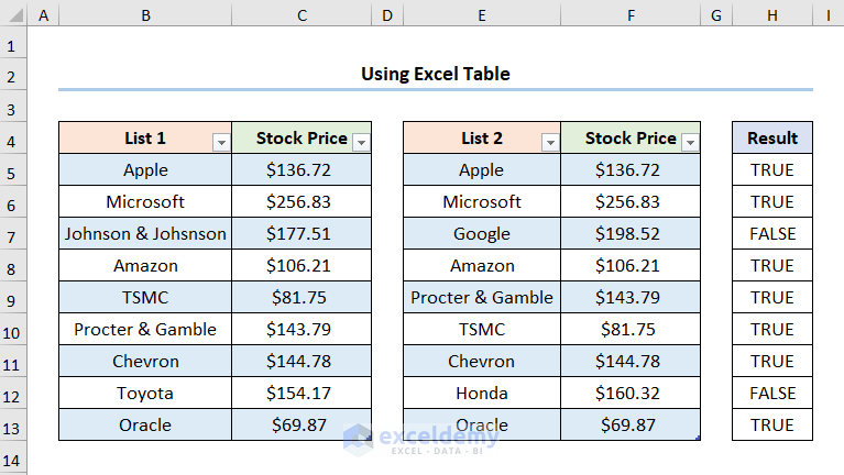
The output should appear as the image below.
Method 6 – Reconciling Two Sets of Data Using the VLOOKUP Function
Steps:
- Go to cell H5 and enter the following formula:
=ISTEXT(VLOOKUP(E5,$B$5:$B$13,1,FALSE))
In this expression, the E5 cell points to the value Apple while the B5:B13 range represents the List 1 array.
⚡ Formula Breakdown:
- VLOOKUP(E5,$B$5:$B$13,1, FALSE) → looks for a value in the left-most column of a table and then returns a value in the same row from a column you specify. Here, E5 ( lookup_value argument) is mapped from the $B$5:$B$13 (table_array argument) array. Next, 1 (col_index_num argument) represents the column number of the lookup value. Lastly, FALSE (range_lookup argument) refers to the Exact match of the lookup value.
- Output → Apple
- ISTEXT(VLOOKUP(E5,$B$5:$B$13,1,FALSE)) → becomes
- ISTEXT(Apple) → The ISTEXT function checks whether a value is text and returns TRUE or FALSE. Here, Apple is the value argument, and since it is a text string, the function returns TRUE.
- Output → TRUE
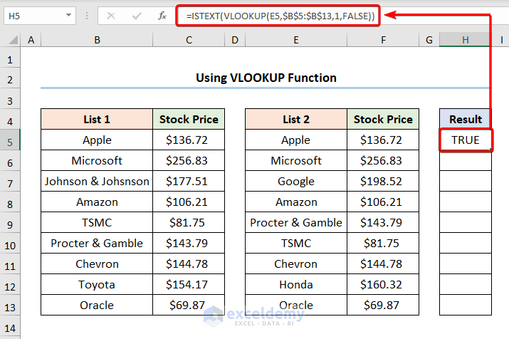
- Copy the formula to the cells below; the results should look like the picture below.

Read More: How to Perform Bank Reconciliation Using VLOOKUP in Excel
Method 7: Applying the XLOOKUP Function
Steps:
- Go to cell H5 and enter the following formula:
=ISTEXT(XLOOKUP(E5,$B$5:$B$13,$B$5:$B$13))
Here, the E5 cell points to the value Apple while the B5:B13 range represents the List 1 array.
⚡ Formula Breakdown:
- XLOOKUP(E5,$B$5:$B$13,$B$5:$B$13) → searches a range or an array for a match and returns the corresponding item from a second range or array. By default, an exact match is used. Here, E5 ( lookup_value argument) is mapped from the $B$5:$B$13 (lookup_array argument) array. Lastly, $B$5:$B$13 (return_array argument) represents the returned array or range.
- Output → Apple
- ISTEXT(XLOOKUP(E5,$B$5:$B$13,$B$5:$B$13)) → becomes
- ISTEXT(Apple) → checks whether a value is text and returns TRUE or FALSE. Here, Apple is the value argument, and since it is a text string the function returns TRUE.
- Output → TRUE
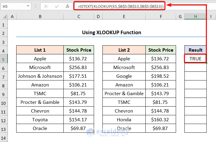
- Copy the formula to populate the cells below; the results should look like the screenshot below.

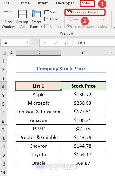
Method 8 – Using the View Side by Side Option to Reconcile Two Sets of Data in Separate Workbooks
Steps:
- Go to the View tab >> click the View Side by Side option.
This opens the Compare Side by Side dialog box.
- Choose the other workbook from the list with which you want to compare the current workbook.
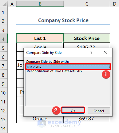
This opens the two workbooks side by side to compare and reconcile their differences.
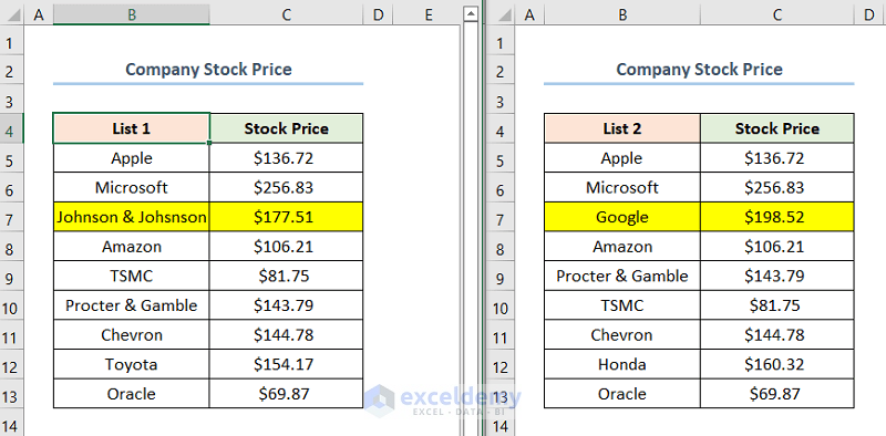
We’ve highlighted the first difference between the two datasets, as shown in the image below.
Method 9 – Reconciling Two Sets of Data in the Same Workbook with a New Window Option
Steps:
- Go to the List 1 worksheet >> go to the View tab >> click the New Window option.
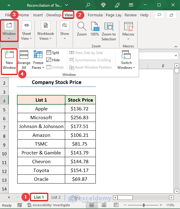
Excel opens a new instance of the same worksheet, as shown in the picture below. In this case, we chose to open the List 2 worksheet in the second instance.
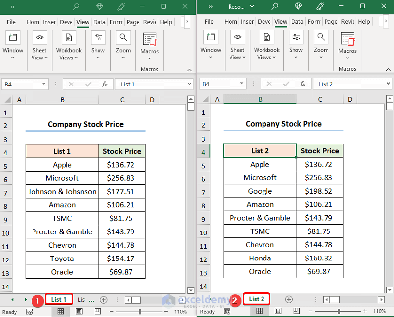
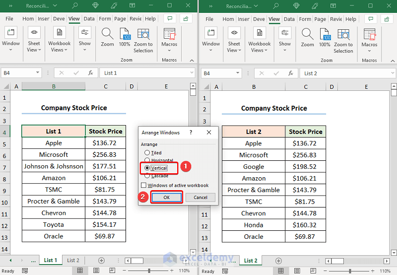
- Go to the View tab >> click the Arrange All option.
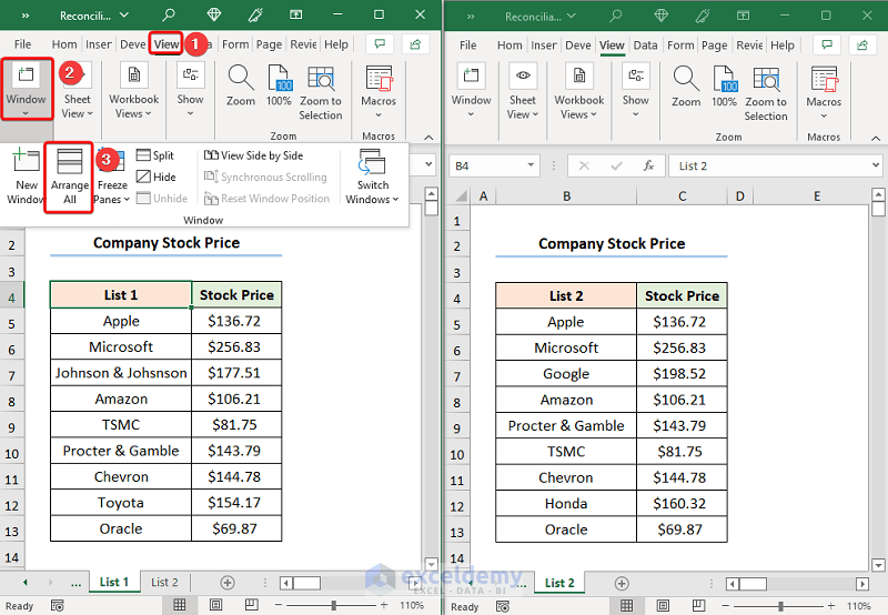
The Arrange Windows dialog box pops up.
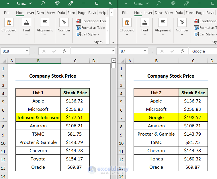
- Choose the Vertical option.
We can highlight the differences between the two datasets, as shown in the screenshot below.
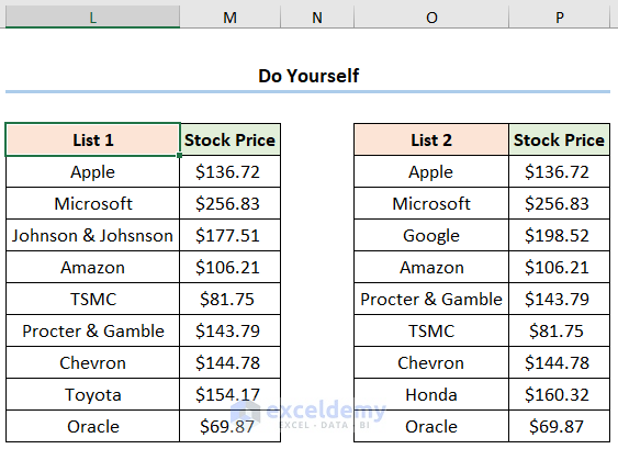
Practice Section
We have provided a Practice section on the right side of each sheet so you can practice.
Download the Practice Workbooks
You can download the practice workbook from the link below.
Related Articles
- How to Do Intercompany Reconciliation in Excel
- Automation of Bank Reconciliation with Excel Macros
- How to Reconcile Vendor Statements in Excel
- How to Do Bank Reconciliation in Excel
- How to Reconcile Credit Card Statements in Excel
<< Go Back to Excel Reconciliation Formula | Excel for Accounting | Learn Excel
Get FREE Advanced Excel Exercises with Solutions!
