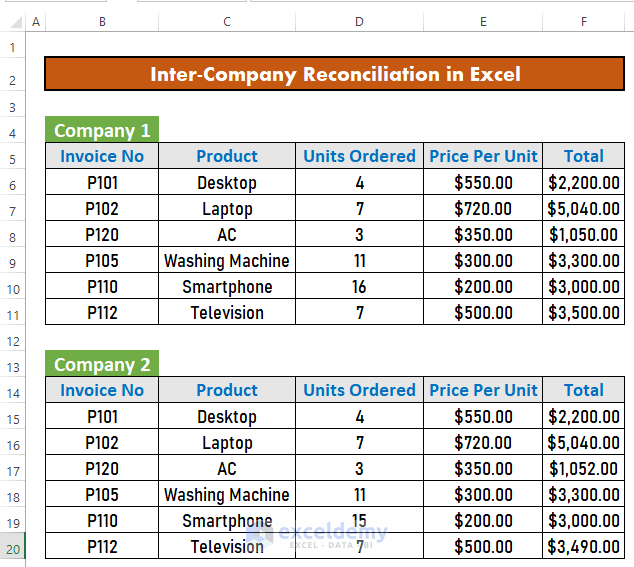
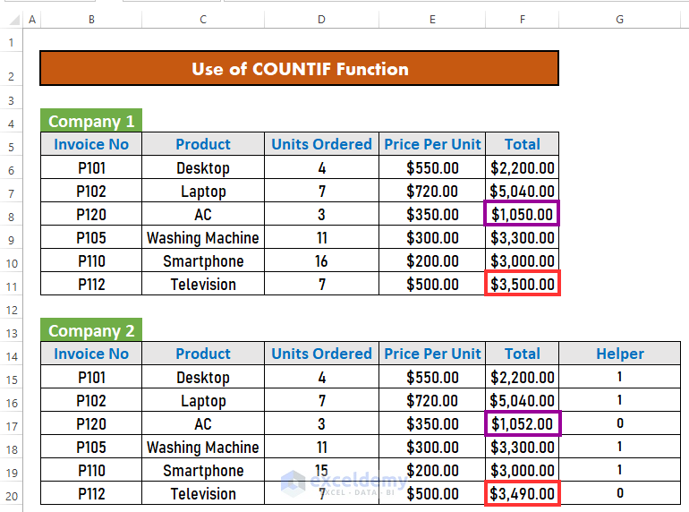
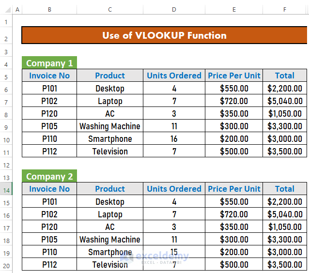
How to Do Intercompany Reconciliation in Excel

The sample dataset showcases transactions in the book of Company 1 and Company 2. Products have Invoice No, Price per Unit, and Total price.

Method 1 – Using the COUNTIF Function to Perform Intercompany Reconciliation

Steps:

To check whether data of Company 2 matches Company 1:

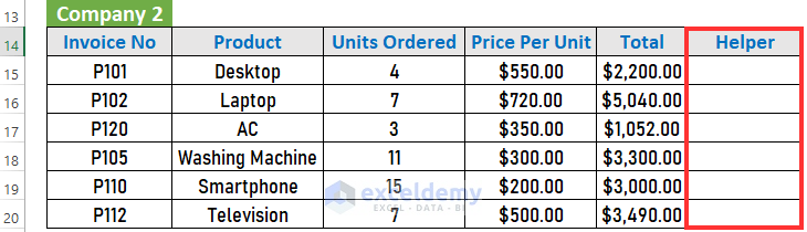
Add a Helper column to the table of Company 2.

Go to G15 and enter the following formula.

=COUNTIF($F$15:$F$20,F6)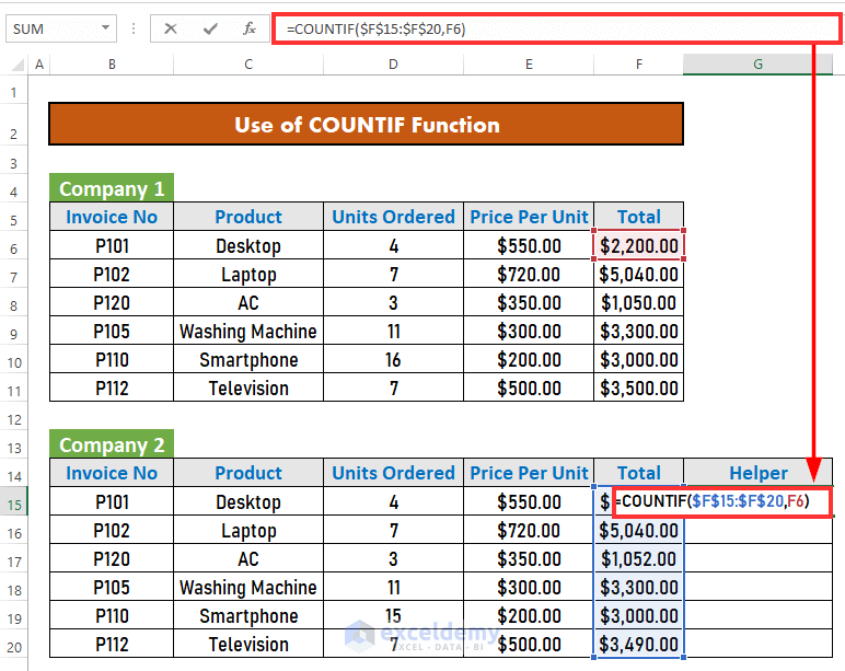

Press ENTER. If there’s a data match, Excel will return 1. If there is any discrepancy, the output will be 0.

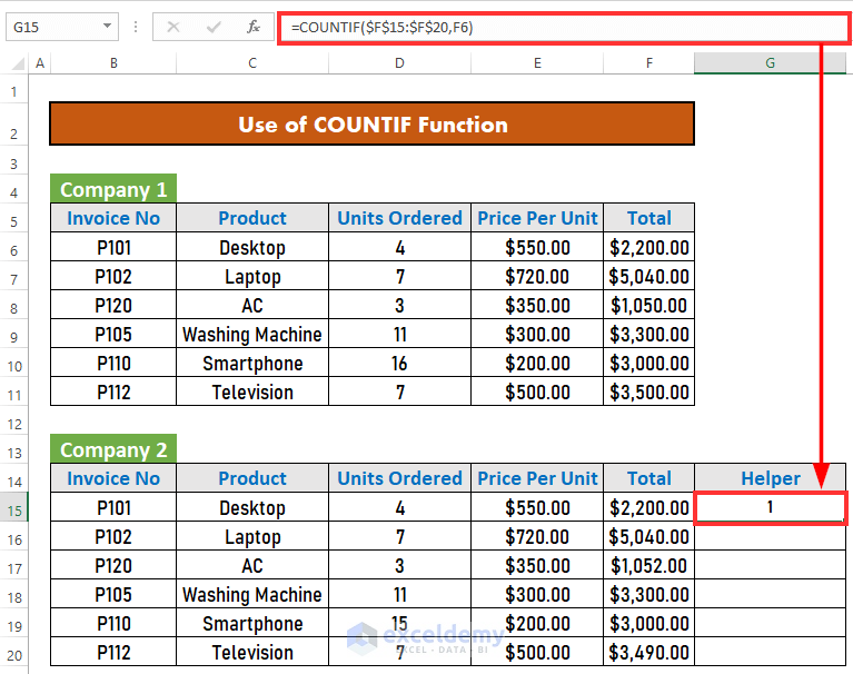
Drag down the Fill Handle to see the result in the rest of the cells.

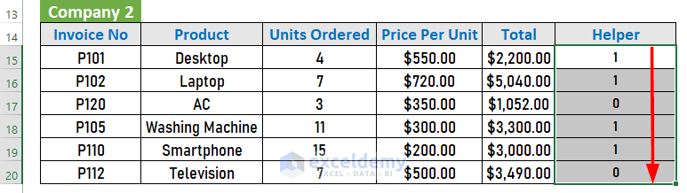
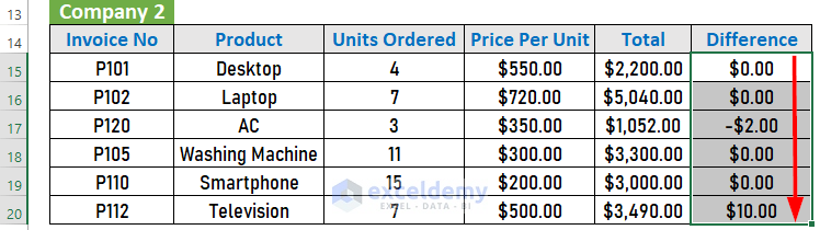
In F17, and F20 the output is 0, as there is no match.

To reconcile data, considering the data of Company 1 as correct, rectify the Company 2 dataset.
To hide the helper column, select it.

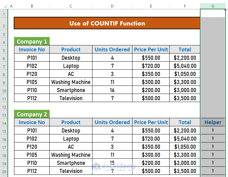
Press CTRL+0.

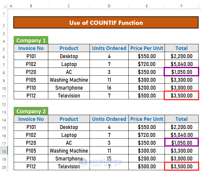
This is the output.

Method 2 – Applying the VLOOKUP Function to perform Intercompany Reconciliation

Steps:

Go to G14 and enter the following formula.

=VLOOKUP(B15,$B$6:$F$11,5,FALSE)-F15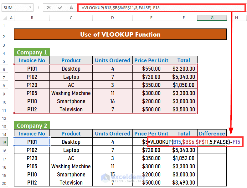

Formula Breakdown:

VLOOKUP(B15,$B$6:$F$11,5,FALSE) → looks for B15 in the array B6:F11. If it finds the value, it will return the corresponding value from the 5th column of the array.
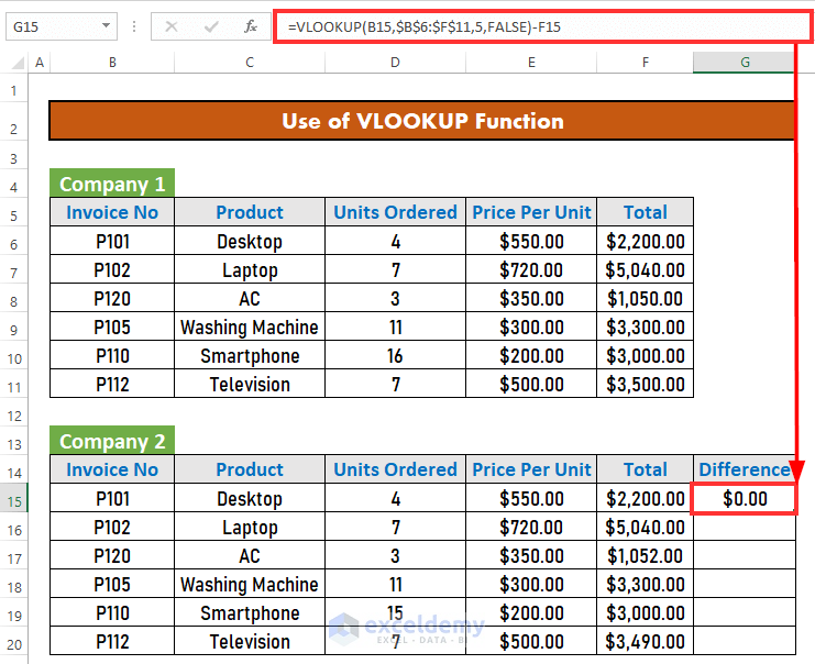
- Output → 2200