Automation of Bank Reconciliation with Excel Macros

Banking reconciliation statements summarize bank and business activity. Using financial records and bank accounts, they reconcile a company’s finances. If you are looking for some special tricks to create a bank reconciliation statement in Excel with VBA Macros, you’ve come to the right place. There is one of the easiest ways to create a bank reconciliation using VBA Macros in Excel. Today, in this article, we’ll learn three quick and suitable steps to make a bank reconciliation in Excel with automation macros effectively with appropriate illustrations.

Introduction to Bank Reconciliation in Excel

It involves comparing and coordinating data from our accounting records with that displayed on a bank statement. The goal is to identify and fix any potential issues, notify the bank immediately if they made a mistake, and fix the discrepancy on our end. Timing discrepancies are unavoidable because you might have written a check on August 5 and the bank might have cleared it on August 6. A manual bank reconciliation takes a lot of time and is prone to mistakes. Excel offers a simple and efficient way to carry out the task. We illustrate how to create bank reconciliation using stacked “for… next” loops in VBA Macros.

Automation of Bank Reconciliation with Excel Macros: 3 Quick Steps

Let’s say, we have a dataset that contains information about several Transactions. Our dataset contains the Cheque Book Number, Withdrawal Amount, and corresponding Date. Using automation Macros, we will create a Bank Reconciliation. Here’s an overview of the dataset for today’s task.

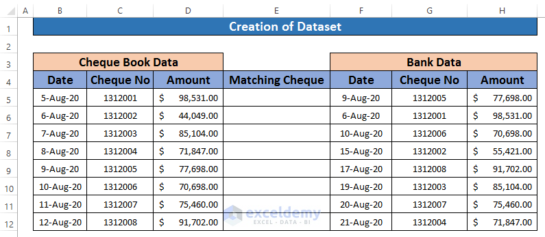
Step 1: Create Dataset with Proper Parameters

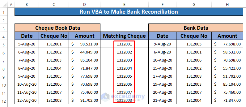
In this section, we will create a dataset to make a Bank Reconciliation using VBA Macros in Excel. We will make a dataset that contains information about several Transactions. Our dataset contains the Cheque Book Number, Withdrawal Amount, corresponding Date, and so on. We will match the Cheque Book Number from the Bank data with Cheque Book data using the VBA Macros. So, our dataset becomes.

Step 2: Open Visual Basic Window

Now, we will enable macros to apply the VBA code. From our dataset, we can easily do that. Let’s follow the instructions below to learn!

First of all, press Alt + F11 from your keyboard.

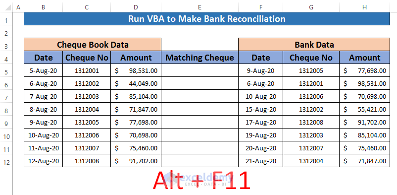
As a result, a window named Microsoft Visual Basic for Applications – Bank Reconciliation will instantly appear in front of you. From that window, we will insert a module for applying our VBA code. To do that, go to,

Insert → Module

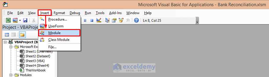
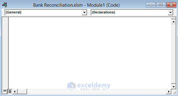
Hence, the Bank Reconciliation module pops up.

Step 3: Run Macros to Create Bank Reconciliation

In this section, we will run the VBA code to make the Bank Reconciliation. From our dataset, we will match the Cheque Book Number from the Bank data with Cheque Book data using the VBA Macros. Let’s follow the instructions below to create a bank reconciliation in Excel with automation macros!

Now, write down the below VBA code in the Bank Reconciliation The VBA code is,

Sub Bank_Reconciliation()
Dim R, M As Integer
For R = 5 To 12
For M = 5 To 12
If Cells(R, 3) = Cells(M, 7) And Cells(R, 4) = Cells(M, 8) Then
Cells(R, 5) = Cells(M, 7)
End If
Next M
Next R
End Sub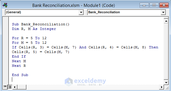

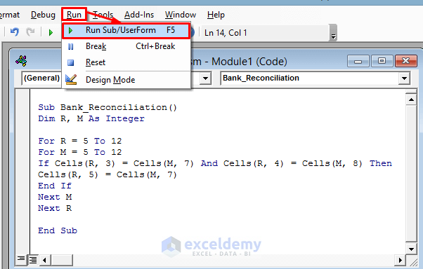
Hence, run the VBA To do that, go to,

Run → Run Sub/UserForm

After running the VBA Code, you will be able to match the Cheque Book number from Bank data with Cheque Book Data which has been given in the below screenshot.

Things to Remember

➜ If a Developer tab is not visible in your ribbon, you can make it visible. To do that, go to,

File → Option → Customize Ribbon

➜ While a value can not found in the referenced cell, the #N/A! error happens in Excel.

➜ #DIV/0! error happens when a value is divided by zero(0) or the cell reference is blank.

Download Practice Workbook

Download this practice workbook to exercise while you are reading this article.

Bank Reconciliation with Macros.xlsm

Conclusion

I hope all of the suitable methods mentioned above to calculate the bank reconciliation will now provoke you to apply them in your Excel spreadsheets with more productivity. You are most welcome to feel free to comment if you have any questions or queries.

<< Go Back to Excel Reconciliation Formula | Excel for Accounting | Learn Excel

Get FREE Advanced Excel Exercises with Solutions!

2 Comments

Philip Earland May 4, 2023 at 10:59 PM

Thankyou for this very useful help. However I need to reconcile debit and credits transferred between differing bank accounts, where the date of transfer is not always the same as transfers do not take place in UK during weekends and public holidays.

Many thanks

Phil
- Reply
  Eshrak Kader May 7, 2023 at 5:11 PM
  
  Hello Philip Earland,
  
  Thank you for your query. You can find the answer to your question in the Excel file linked to this message. The steps are described below.
  Bank Reconciliation.xlsx
  
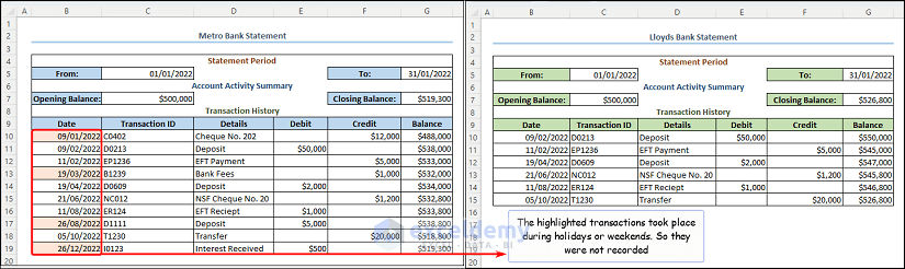
  Consider the transactions from “Metro Bank” to “Lloyds Bank”. We can see the closing balances are not the same and need to be reconciled.
  
  Select the transaction dates in the B10:B19 cells >> click the Conditional Formatting drop-down >> go to New Rule.
  
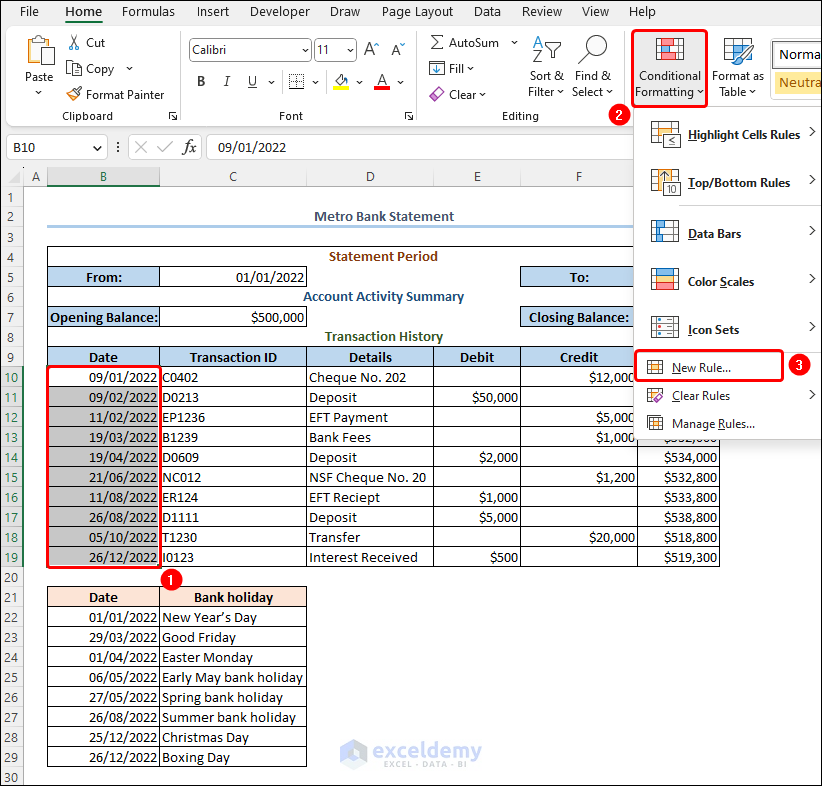
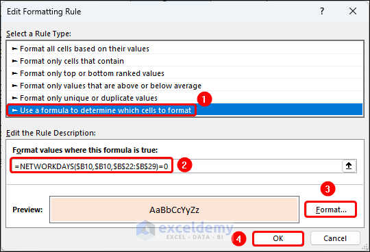
  Select Use a formula to determine which cells to format option >> enter the formula given below >> select fill color, here we’ve chosen the color “Orange, Accent 2, Lighter 80%”.
  =NETWORKDAYS($B10,$B10,$B$22:$B$29)=0
  
  Here, the highlighted transactions were processed by “Metro Bank” just before the weekends or holidays, so they were not recorded in the “Lloyd Bank” statement.
  
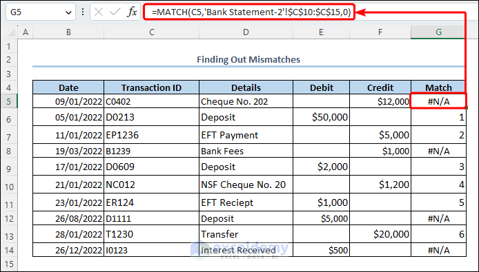
  Next, move to the “Mismatch” worksheet and apply the MATCH function to find the discrepancies between the two statements. Here the #N/A errors are the mismatches.
  
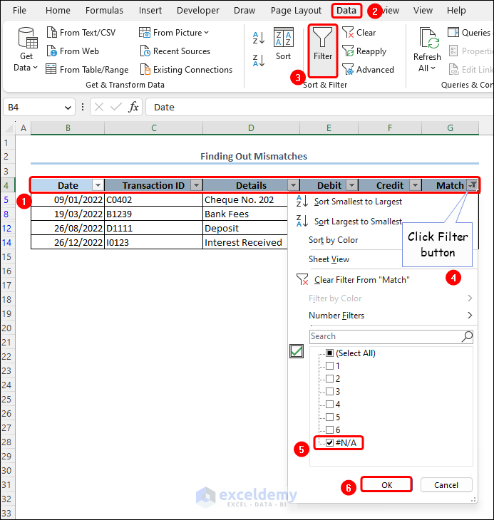
  Then, use the Filter option in the Data tab to show only the mismatches.
  
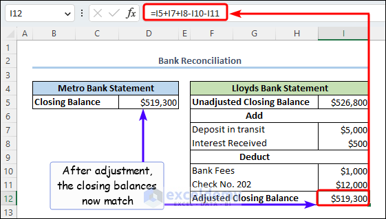
  Enter the mismatched account names and their amounts >> apply the expression below to reconcile the differences.
  =I5+I7+I8-I10-I11
  
  Hope this helps. Have a good day.
  
  Regards,
  Exceldemy