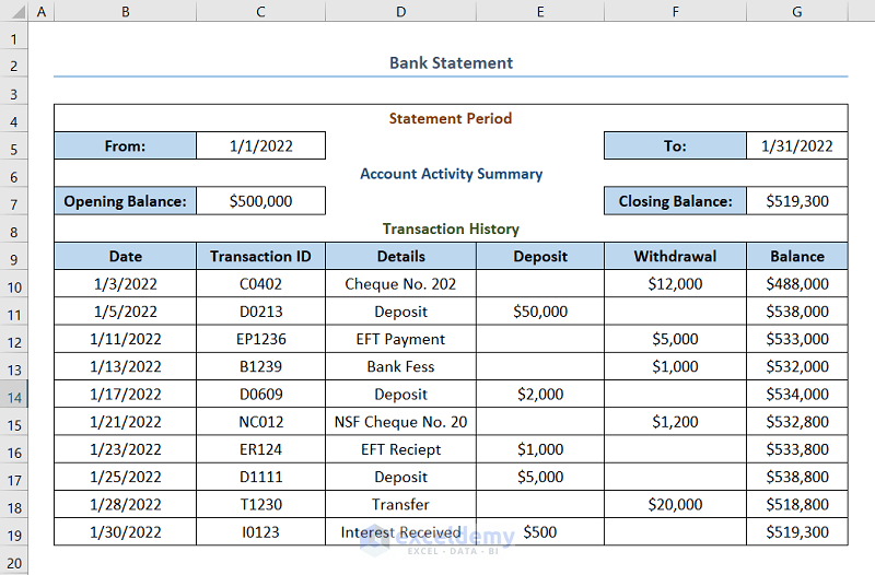
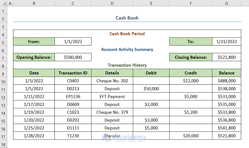
How to Do Bank Reconciliation in Excel (with Easy Steps)

Let’s assume you have a Bank Statement and a Cash Book as shown below. Here, we can see that the closing balances don’t match. So, you want to do Bank Reconciliation. In Microsoft Excel, you can easily do Bank Reconciliation by following these steps.

⭐ Step 1 – Find Mismatches in Bank Statement and Cash Book

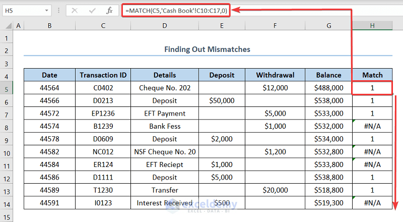
Take the Transaction History from the Bank Statement and copy it to another blank sheet.
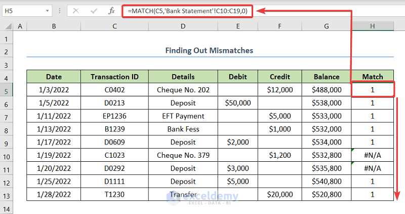
Select cell H5 and insert the following formula.

=MATCH(C5,'Cash Book'!C13:C20,0)

In this case, cells H5 and C5 are the first cell of the column Match and Transaction ID. Also, Cash Book is the worksheet name that contains the Cash Book.

Drag the Fill Handle for the rest of the cells.

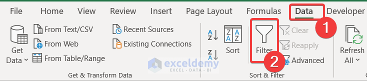
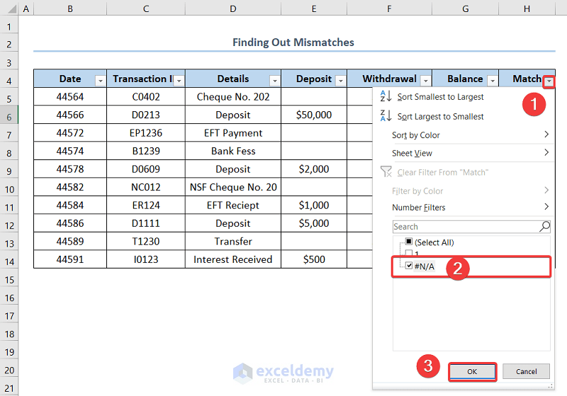
You will use Sort & Filter to find out the mismatches of the Bank Statement with the Cash Book.

Go to the Data tab.
Click on Filter.

Click on the arrow sign in the column heading Match.
Select #N/A.
Click OK.

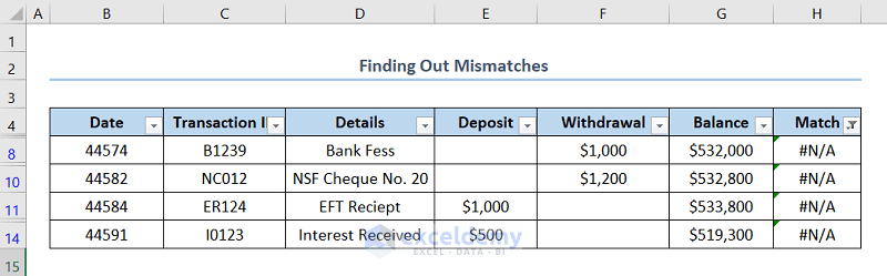
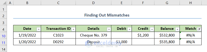
You will get the mismatches in the Bank Statement with the Cash Book.

Take the Transaction History from the Cash Book and copy it to another blank sheet.
Select cell H5 and insert the following formula.

=MATCH(C5,'Bank Statement'!C15:C24,0)

In this case, cells H5 and C5 are the first cells in the column Match and Transaction ID respectively. Also, Bank Statement is the worksheet name which contains the Cash Book.

Drag the Fill Handle for the rest of the cells.

Sort and filter the data as shown above to find out the mismatches in the Cash Book with the Bank Statement.

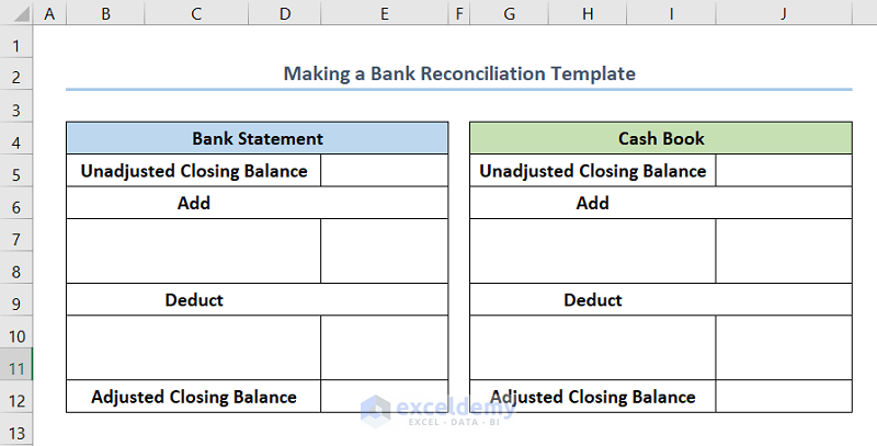
⭐ Step 2 – Make a Bank Reconciliation Template in Excel

In this step, we will make a Bank Reconciliation Template in Excel. You can make a template as shown in the below screenshot on your own or else you can download the practice workbook and get this template.

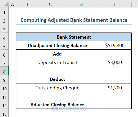
⭐ Step 3 – Compute the Adjusted Bank Statement Balance

Include the data like Deposit in Transit below Add.
Insert the data like Outstanding Cheques below Deduct.

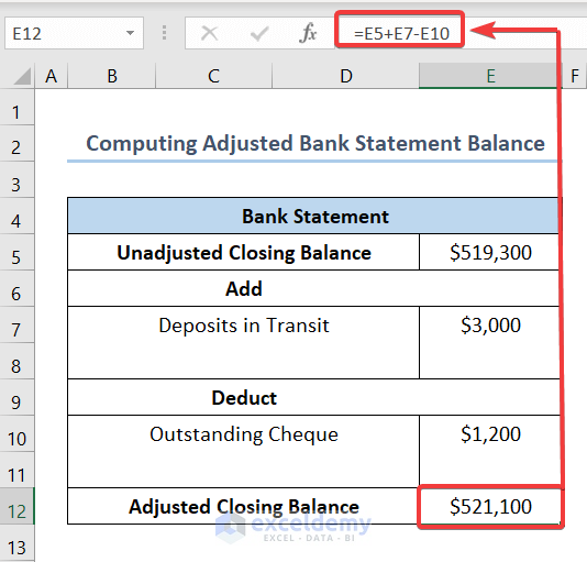
Type the following formula in cell E12.

=E5+E7-E10

In this case, cells E5, E7, E10, and E12 indicate the Unadjusted Closing Balance, Deposit in Transit, Outstanding Cheque, and Adjusted Closing Balance respectively.

Read More: How to Do Reconciliation in Excel

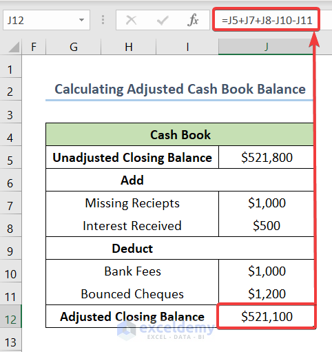
⭐ Step 4 – Calculate Adjusted Cash Book Balance

Include the data like Missing Receipts and Interest Received below Add.
Insert the data like Bank Fees and Bounced Cheques below Deduct.

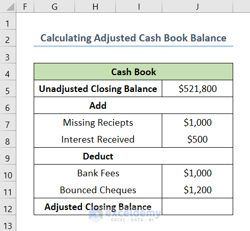
Write the following formula in cell J12.

=J5+J7+J8-J10-J11

In this case, cells J5, J7, J8, J10, J11, and J12 indicate the Unadjusted Closing Balance, Missing Receipts, Interest Received, Bank Fees, Bounced Cheques, and Adjusted Closing Balance respectively.

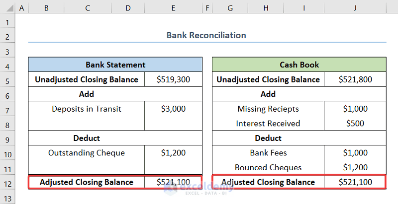
⭐ Step 5 – Match the Adjusted Balances to Do Bank Reconciliation

Match the Adjusted Closing Balances to finish Bank Reconciliation. In the following screenshot, we can see both the balances for Bank Statement and Cash Book match.

Download Practice Workbook

You can download the practice workbook from the link below.

Doing Bank Reconciliation.xlsx

<< Go Back to Excel Reconciliation Formula | Excel for Accounting | Learn Excel

Get FREE Advanced Excel Exercises with Solutions!

2 Comments

Tomás Limeme Apr 18, 2023 at 7:05 PM

Would you add up the reasons on why adding or deducting transactions on balancing the unadjusted balance, so that the reader may have further understanding thereon and avoid doing things mecanically? I know that your article is not an introduction on what is a reconciliation as such, but a practical guideline for those who know it, however there might be readers for whom it may be first time to read about reconciliation. Reasons are the heart of the actions, otherwise people will act inadvertently.
- Reply
  Eshrak Kader Apr 24, 2023 at 3:56 PM
  
  Hello Tomás Limeme,
  
  Thank you for your feedback. The goal of a bank reconciliation is to identify and adjust any difference between the closing balances of our cashbook and bank statement over a specific period. To do this, we add or subtract any unrecorded transaction from our unadjusted closing balance.
  
  In short, adding and subtracting ensures the matching of the bank statement and cashbook balances. This is important for proper financial reporting and to avoid mistakes or fraud.
  
  Let’s review some of the transactions that are added, followed by the transactions that are subtracted.
  
  Examples of transactions that are added include:
  1. Deposits in transit: Funds transferred to the bank account but not yet entered into the accounting system.
  2. Bank errors: Mistakes made by the bank, such as incorrectly recorded deposits or credits.
  3. Earned interest: Interest on an account that hasn’t been entered into the accounting system.
  
  On the other hand, subtracted transactions are:
  1. Outstanding checks: Checks that have been written but have not yet been cashed by the bank.
  2. Bank fees: Charges made by banks that are not accounted for in the accounting system.
  3. Not Sufficient Fund checks: Checks that the bank returned due to insufficient money in the account of the issuer.
  
  Hope this helps, have a good day.
  
  Regards,
  ExcelDemy