Suppose you have a list of your daily or monthly transactions. You want to know in which transaction category you are spending the most. You can get this quickly by calculating the percentage of total of every transaction category in Excel.
Overview of Calculating Percentage of Total in Excel using the SUM function and Excel formula
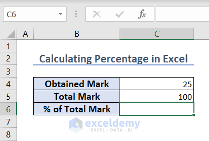
How to Calculate Percentage in Excel
The general formula to calculate percentage is:

In Excel, you can calculate percentage very easily. Consider a dataset like the following image.
Steps:
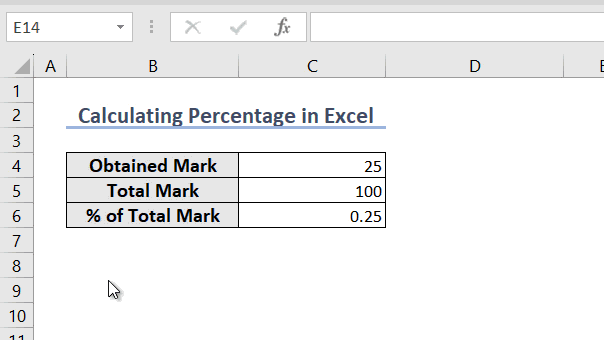
- In cell C6, we want to calculate the Obtained Mark in % of the Total Mark. We’ll input this formula in the cell C6:
=C4/C5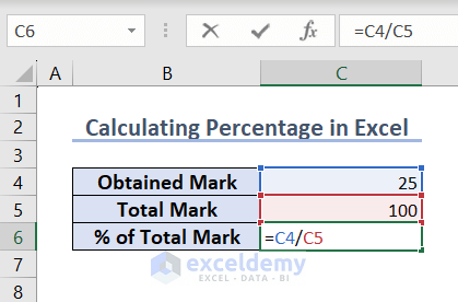
- Hit Enter on your keyboard and you will find the output.
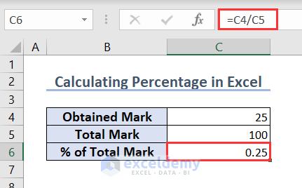
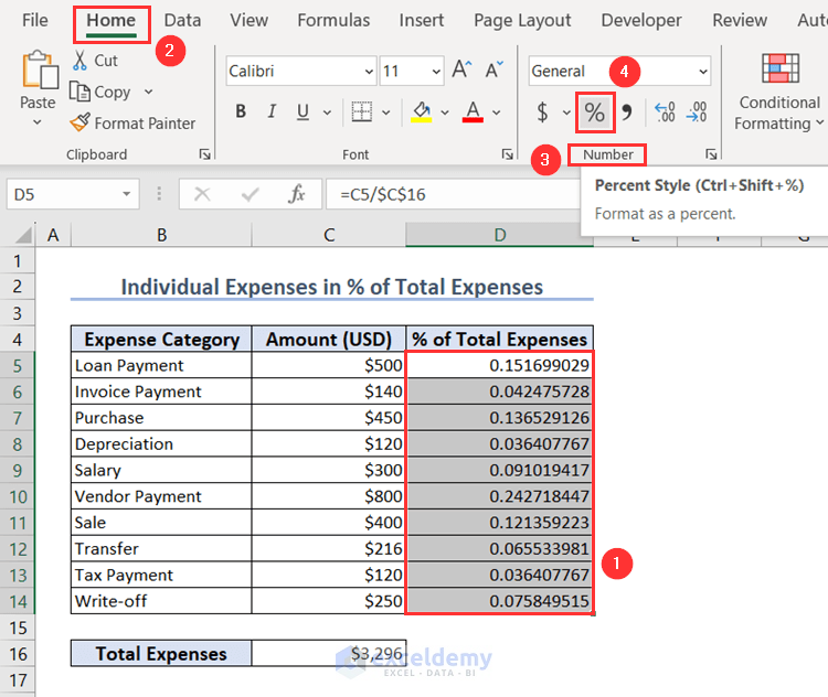
Excel automatically shows the results in decimal values. This is why cell C6 is showing value in decimal. Let’s convert the cell value of C6 to percentage.
- Select the cell C6.
- Go to the Home tab and to the Number group. Select the % icon.
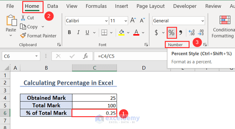
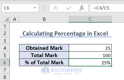
- Here’s the result.
You can also use the keyboard shortcut Ctrl + Shift + 5 on a cell.
Method 1 – Using SUM Function and Excel Formula to Calculate Percentage of Total
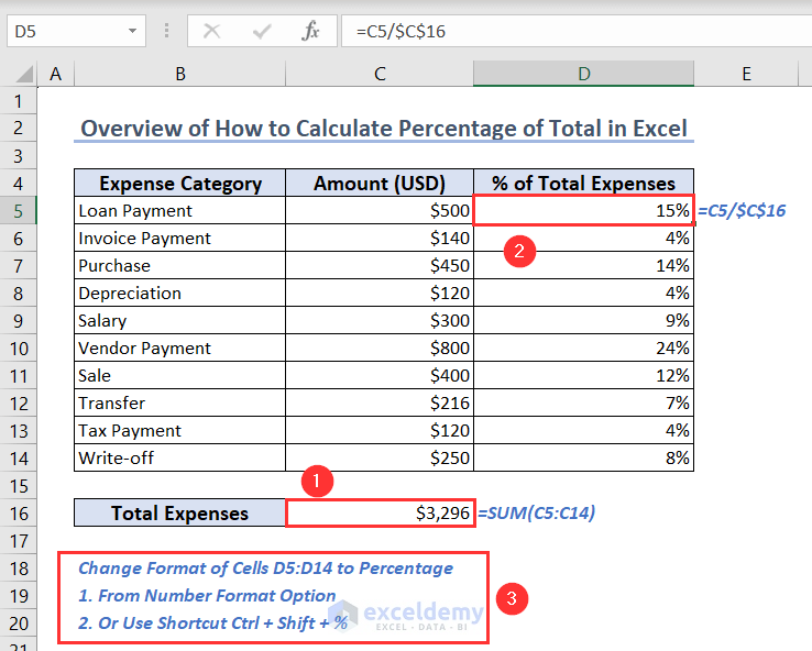
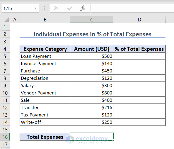
Example 1 – Find Individual Category Expenses in % of Total Expenses
Here’s a dataset with individual Expense Category and Amount. We want to find the Individual Category Expenses in % of the Total Expenses.
Steps:
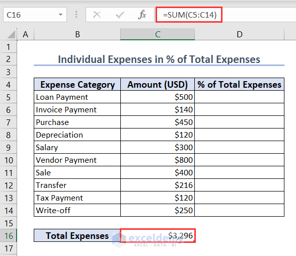
- In cell C16, we want to calculate the total expenses. So, we input this formula in cell C16:
=SUM(C5:C14)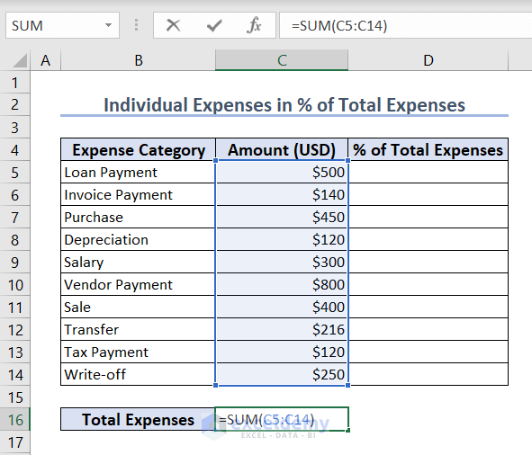
- Hit the Enter key and you will find the following output.
- In cell D5, we want to calculate the individual expenses in % of total expenses. So, we’ll input this formula in the cell:
=C5/$C$16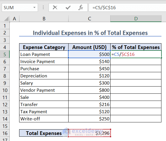
- Hit Enter.
- Hover your mouse over the bottom right corner of cell D5, you will find the Fill Handle icon (Plus).
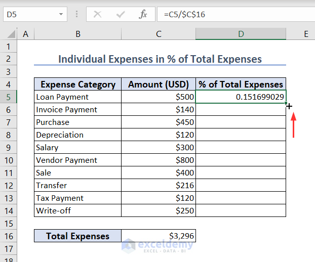
- Double-click on the Fill Handle icon to obtain all the individual expenses in % of total expenses across cells D5:D14.
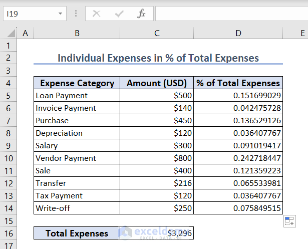
- Convert the values to percentages with the % icon in the ribbon or Ctrl + Shift + 5.
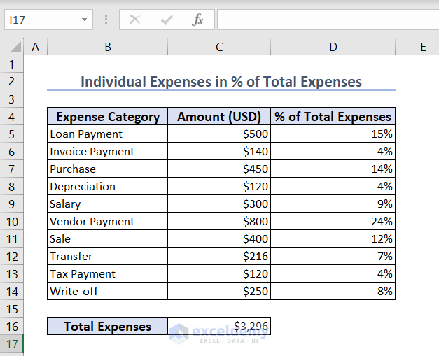
- You will get the following result.
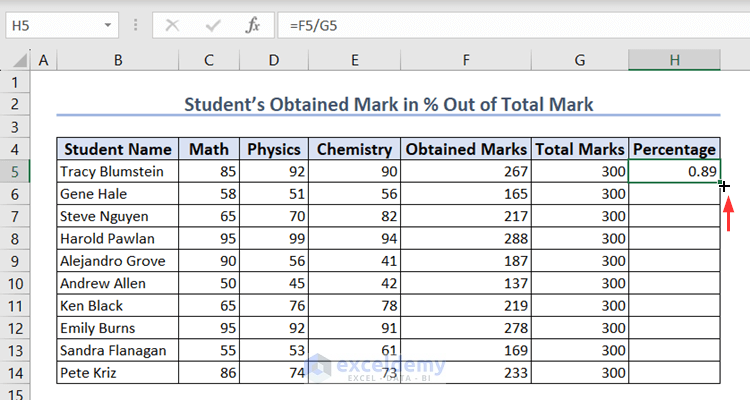
Example 2 – Find an Individual Student’s Obtained Mark in % Out of Total Mark
Consider this dataset with student marks. It has marks in 3 subjects and the highest Total Mark of the 3 subjects. We want to find the Individual Student’s Mark in % of the Total Mark.
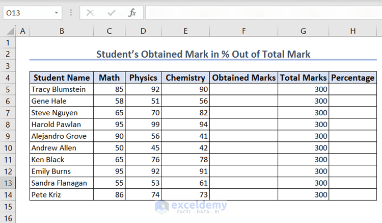
Steps:
- Input this formula in cell F5 to get a student’s total marks:
=SUM(C5:E5)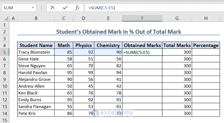
- Hit Enter and hover over the bottom-right corner of the cell.
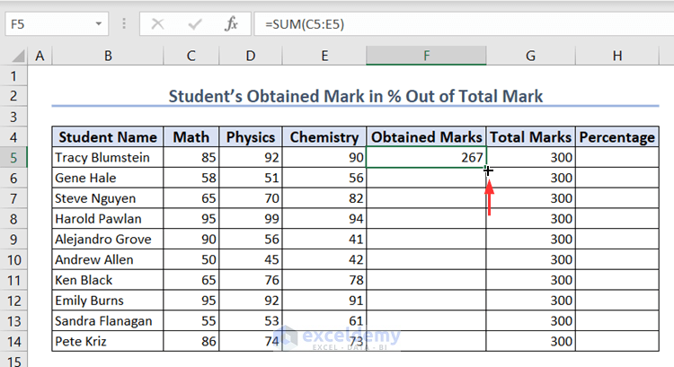
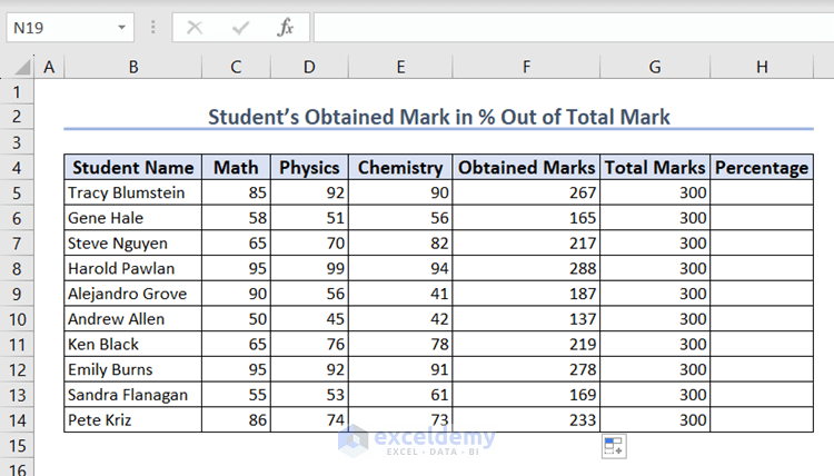
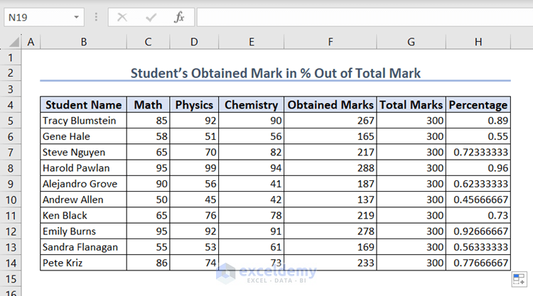
- Double-click on the Fill Handle icon to get the obtained marks of all students across cells F5:F14.
- Input this formula in the cell H5:
=F5/G5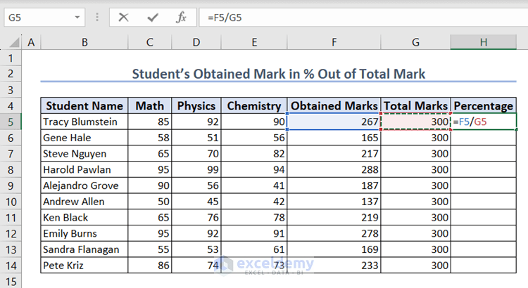
- Apply the formula and drag the Fill Handle to populate the column.
- Here are the results from the sample.
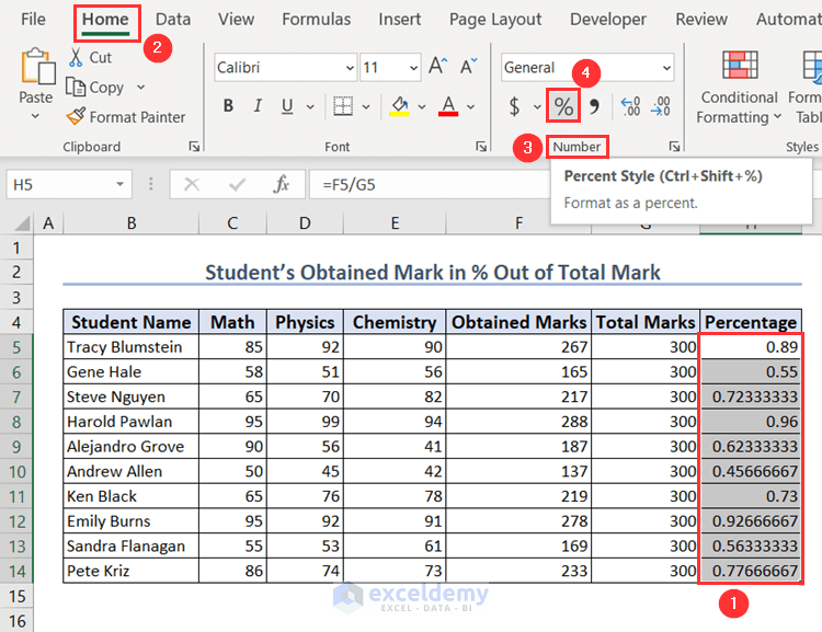
- Convert the cells to a percentage format by selecting the % icon in the Number group from the Home tab.
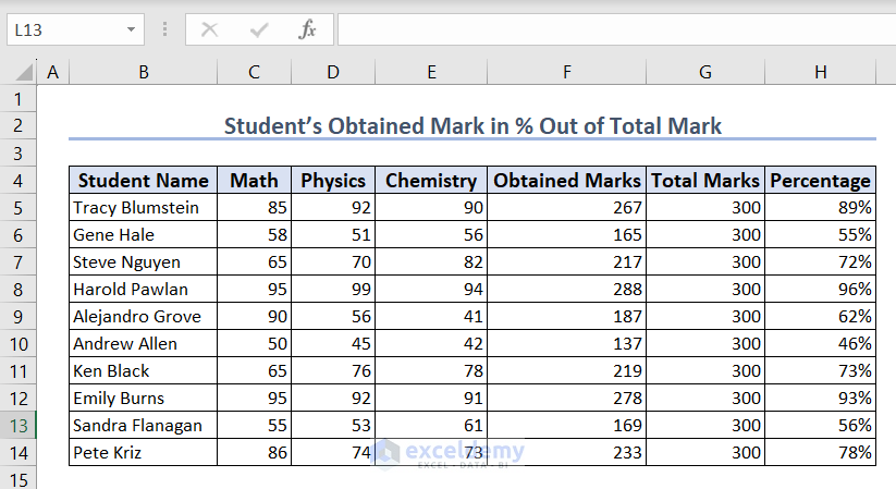
- Here’s the final result.
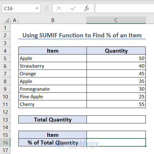
Method 2 – Using SUMIF Function and Excel Formula to Calculate Percentage of Total Quantity of an Item Based on Drop-Down List
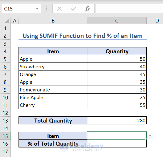
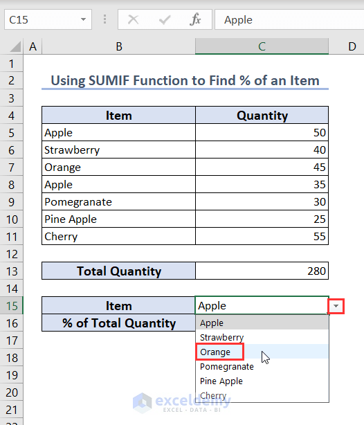
Consider a dataset with Item and Quantity. We’ll put a drop-down list in cell C15 and calculate the % of the Total Quantity of an Item in cell C16. When I select an item from the list, the cell C16 will show the % of the Total Quantity based on that Item.
Steps:
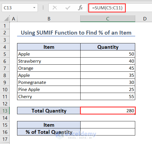
- Input this formula in cell C13 to get the total quantity:
=SUM(C5:C11)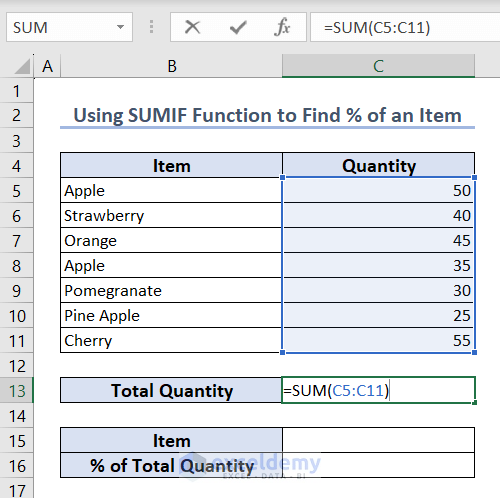
- Hit Enter.
- Select cell C15.
- In the Data tab, go to Data Tools group of commands and select Data Validation.
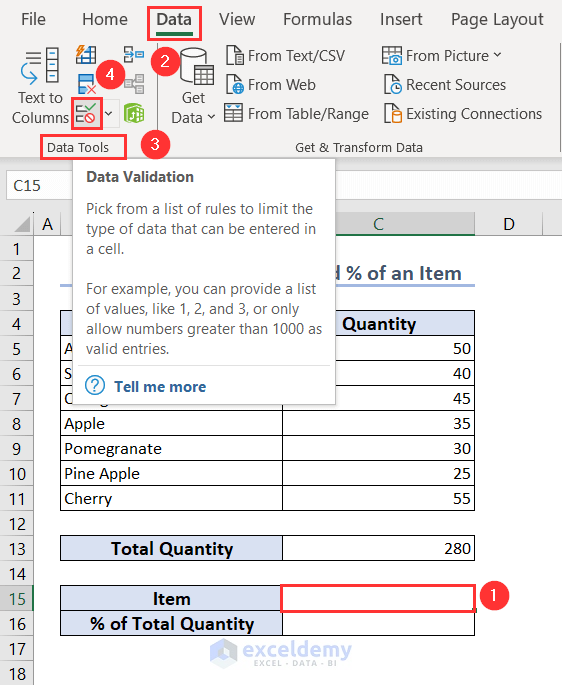
- You will get the Data Validation dialog box
- In the Settings tab, choose List from the Allow drop-down.
- Put this formula =$B$5:$B$11 in the Source box.
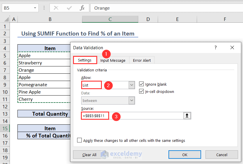
- Click OK.
- Click the drop-down icon to see the list.
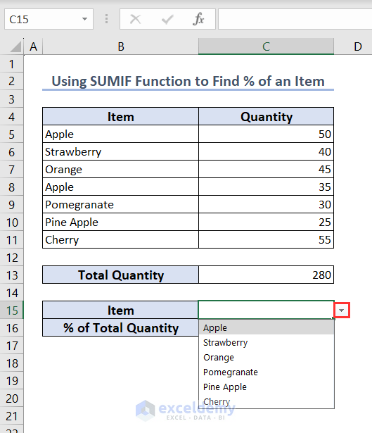
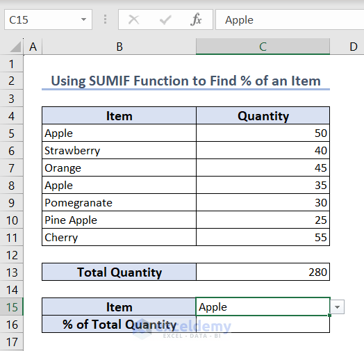
- We selected Apple from the list.
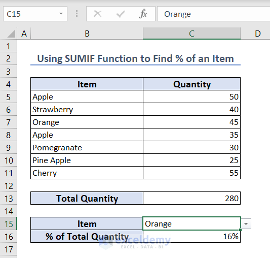
- Input this formula in cell C16:
=SUMIF(B5:B11,C15,C5:C11)/C13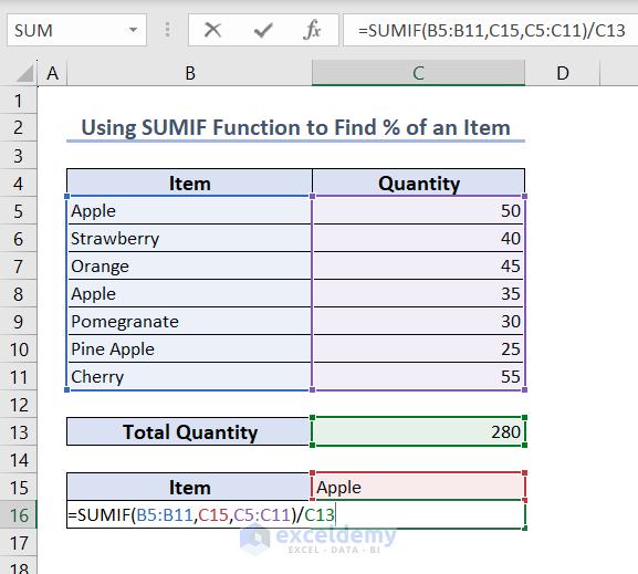
- Hit Enter.
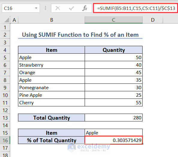
- Select the Percent Style in the Number group (the Home tab).
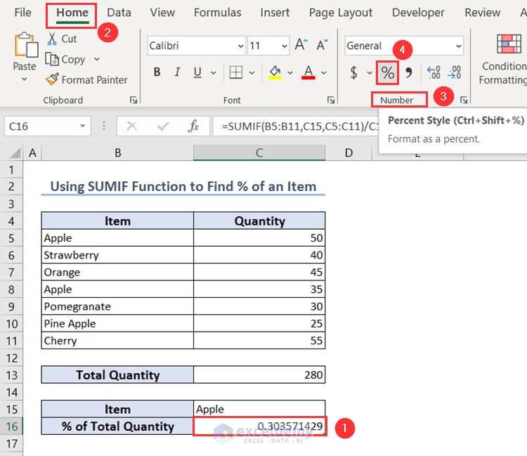
- Click on the Percent Style icon and you will get the following result.
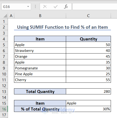
- Click on the drop-down icon and switch to Orange from the drop-down list.
- Selecting Orange from the drop-down list changes the result to the % of the total quantity of Orange automatically.
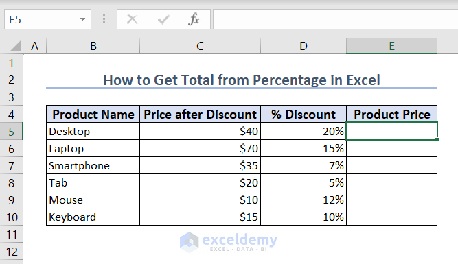
How to Get Total from Percentage in Excel
You can get the total from the percentage in Excel by dividing Part with the Percentage value.
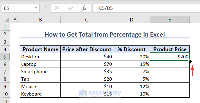
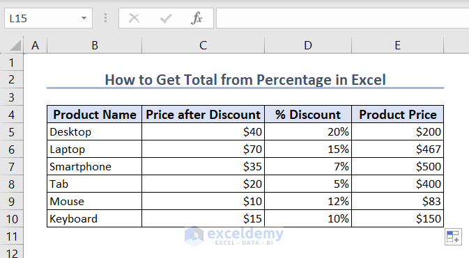
We have a dataset with some Products, their Prices after Discount, and % of Discount. We want to calculate the original Product Price from % of the Discount.
Steps:
- Input this formula in the cell E5:
=C5/D5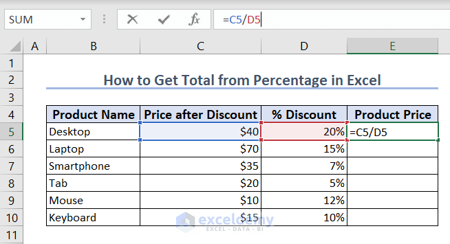
- Hit Enter and hover over the bottom-right corner of the cell to find the Fill Handle.
- Double-click on the Fill Handle icon to get the Product Price of all Products across cells E5:E10.
Download Workbook
Related Articles
- How to Convert Number to Percentage in Excel
- How to Divide a Value to Get a Percentage in Excel
- How to Calculate Reverse Percentage in Excel
- How to Convert Percentage to Number in Excel
- How to Convert Percentage to Whole Number in Excel
- How to Show One Number as a Percentage of Another in Excel
- How to Add a Percentage to a Number in Excel
- Make an Excel Spreadsheet Automatically Calculate Percentage
- Convert Number to Percentage Without Multiplying by 100 in Excel
<<Go Back to Calculating Percentages in Excel | How to Calculate in Excel | Learn Excel
Get FREE Advanced Excel Exercises with Solutions!

I’m hoping you can help with an issue that I am having. I have Column D with a list of totals.The last cell in column D is D13 with the sum(D3:D12). Now I have column E for percent of total volume, this formula =D3/$D$13, =D4/$D$13,=D5/$D$13 and so on (D13 is where I have the Total for column D). To double check that my percent totals add up to 100, the last cell in E =sum(E3:E12) – this is the range that contains the percentages. It does add up to 100% but if I delete a value in column D, the total percent remains at 100% even though the percent for the individual value is now 0% (because I deleted the total for that item). Why isn’t my sum of percent cell updating? 🙁 I can’t figure this out.
Greetings Debbie,
First of all,we really appreciate for your question. Now if I am not afraid, you asked about why your total percentage value not changed despite deleting one sample value. If this is the case, the reason is pretty simple. as you delete one value, your total value also change. Which in turns also change the percentage value of all the other values. and this change will happen in a way that the total percentage values are always sums up to 100, following the basic arithmatic rule.
If this is not the case,please provide your Excel worksheet containing your data and we will have a look.
Thanks and Regards
Rubayed Razib