How to Calculate Reverse Percentage in Excel (4 Easy Examples)

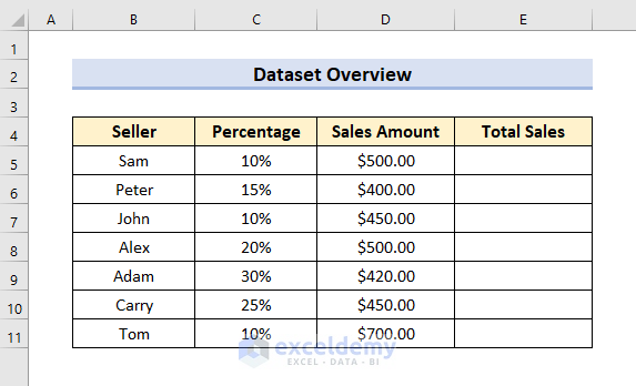
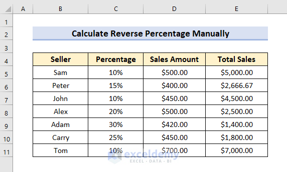
Example 1 – Calculate Reverse Percentage Manually in Excel

We will use the following sample dataset that contains the percentage of the total amount in the Percentage column and the Sales Amount represented by the percentage of some sellers. We will try to find the total sales amount of the sellers.

STEPS:

• Enter the following formula in Cell E5.

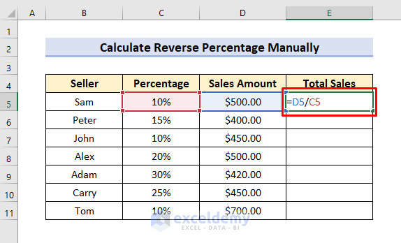
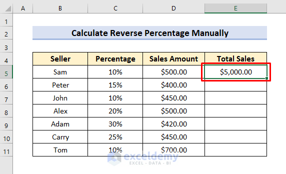
• Press Enter to get the result.

The formula divides the sales amount by the percentage to get the total sales value.

• Use the Fill Handle tool for the remaining cells.

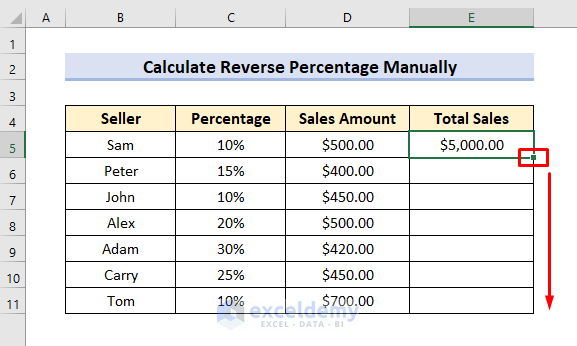
• The result will be as shown in the following image.

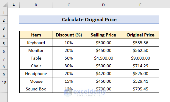
Example 2 – Compute Reverse Percentage to Obtain Original Price

We will calculate the reverse percentage to obtain the original price of some products when discounts are available. We will use a sample dataset that contains the discounts in percentage and the current selling price of some products. We will use a formula to calculate the original price of the products.

STEPS:

• Enter the following formula in Cell E5.

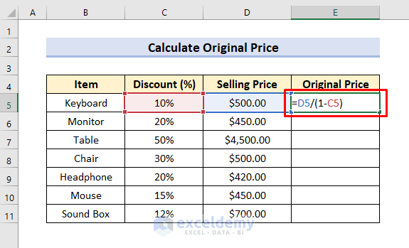
• Press Enter to see the result.

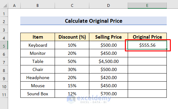
This formula subtracts the discount from 1 and divides the current sales by the subtracted result.

• Use the Fill Handle tool for the remaining cells.

Example 3 – Determine Reverse Percentage in Excel to Find Initial Price

We will determine the initial price in this example. We will use a sample dataset that contains the change in percentage and the current price of some products. The change can be positive or negative. Positive change suggests that the current price of the product is higher than the initial price. Similarly, negative change means that the current price of the product is lower than the initial price.

STEPS:

• Enter the following formula in Cell E5.

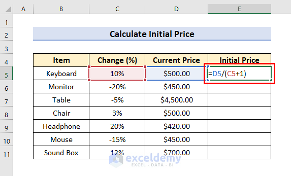
• Press Enter to see the result.

The formula added the value of change with 1 and divided the current price by it to find the initial price.

• Use the Fill Handle tool for the remaining cells.

Example 4 – Excel MROUND Function to Calculate Reverse Percentage

We can use the MROUND function to display the reverse percentage in a rounded figure. The MROUND function returns a number rounded to the desired multiple. To explain this example, we will use the dataset of Example-1.

STEPS:

• Enter the following formula in Cell E5.

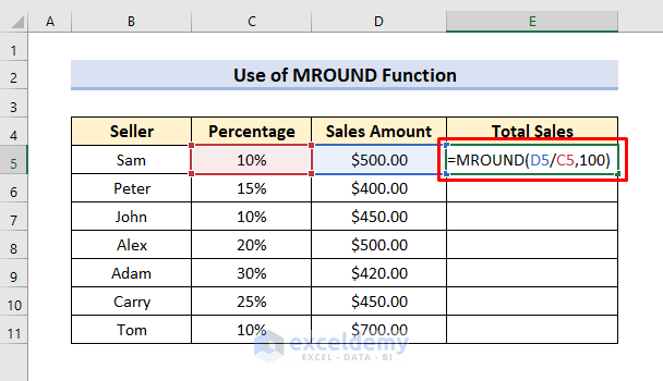
• Press ENTER.

The MROUND function first calculates the ratio of sales amount and percentage, after which it returns a number to the multiple of 100.

• Use the Fill Handle tool for the remaining cells.

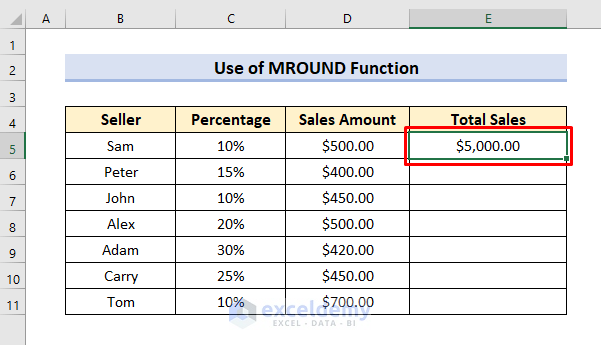
In the Cell E6, you will notice the total sales value is different from the value we got in Example 1. We got $2,666.67 in the first example but $2700.00 in this example. The MROUND function has rounded the value to the multiple of 100.

Download Practice Book

Related Articles

• How to Calculate Percentage of Total in Excel
• How to Convert Number to Percentage in Excel
• How to Find the Percentage of Two Numbers in Excel
• How to Divide a Value to Get a Percentage in Excel
• How to Convert Percentage to Number in Excel
• How to Convert Percentage to Whole Number in Excel
• How to Show One Number as a Percentage of Another in Excel
• How to Add a Percentage to a Number in Excel
• Make an Excel Spreadsheet Automatically Calculate Percentage
• Convert Number to Percentage Without Multiplying by 100 in Excel

<<Go Back to Calculating Percentages in Excel | How to Calculate in Excel | Learn Excel