Latest Posts From Mursalin Ibne Salehin

Method 1 - Calculate BMI in Metric Unit Select cell E5 and type the following formula: =D5/C5^2 D5 is the weight, and C5 is a person's height. Both ...
What Is a Chart in Excel? Charts in Excel serve as powerful tools for visually representing data. Whether you’re analyzing sales figures, tracking trends, or ...

Cell Borders in Excel: Knowledge Hub How to Insert Border in Excel How to Apply All Borders in Excel How to Apply Top and Bottom Border in Excel ...

The sample dataset contains the Department and Joining Month of some employees in the range B4:D10. In the empty cells, we need to copy the above cell. ...
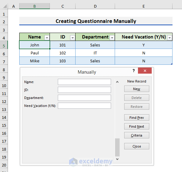
Method 1 - Creating a Questionnaire Manually in Excel STEP 1: Insert Keywords of Questions We need to identify the keywords of the questions and put them ...

This is the sample dataset. Method 1 - Converting Single Alphabet letters to Numbers in Excel 1.1 Using the COLUMN Function STEPS: Select ...
How to Extract Data from XML to Excel: 2 Easy Ways We will extract data from the XML file to Excel using both the Data and Developer tabs. Method 1 ...

In this article, we will demonstrate anchoring the comment boxes in Excel. Anchoring comment boxes in a specific location is a tricky task. In Excel 365, ...

In this article, we will learn to calculate the variance inflation factor in Excel. It is also expressed as VIF. Variance Inflation Factor or VIF detects the ...

In this article, we will learn to find the Discrete Probability Distribution in Excel. A discrete probability distribution indicates the probability of the ...

In this article, we will learn to create a real estate balance sheet in Excel. A real estate balance sheet is a financial report that reflects the net worth of ...

In this article, we will learn to perform floating rate bond valuation in Excel. The floating rate bond pays coupons that vary over their maturity. The ...

In this article, we will learn to use ANOVA two factor without replication in Excel. Microsoft Excel is a powerful tool and makes complicated calculations ...
Introduction to Excel CHOOSE Function The CHOOSE function requires two arguments: index_num and value1, along with optional additional values. ...
What Is Average Daily Balance? The Average Daily Balance method is a way to find the interest or finance charge on a credit card. To calculate the average ...
- 1
- 2
- 3
- …
- 11
- Next Page »
See Our Reviews at


Hi JUN,
Thanks for your comment. I assume you are having this problem because Excel considers 1 (‘dataset’!=”1″) as a number. You don’t need to add the double quotation symbol for that part. So, an error occurs and it is showing “–” instead of “A“. You can use the formula below to get “A“:
=IFERROR((INDEX(datasheet!C:C,MATCH(1,(datasheet!A:A=1)*(datasheet!B:B="a")*(datasheet!D:D="22/8/1"),0))),"-")To get “B“, use the formula below:
=IFERROR((INDEX(datasheet!C:C,MATCH(1,(datasheet!A:A=2)*(datasheet!B:B="b")*(datasheet!D:D="22/8/1"),0))),"-")And to get “C“, you can use the formula below:
=IFERROR((INDEX(datasheet!C:C,MATCH(1,(datasheet!A:A=3)*(datasheet!B:B="c")*(datasheet!D:D="22/8/1"),0))),"-")For your convenience, I have attached the excel file below with the formulas that I have used. I have used the formulas in Excel 365.
Download Excel File
I hope this will help you to solve your problem. If you still find any problem in your excel file, then you can send it to [email protected]. I will take a look and email you the solution.
Thanks!
Hi RICK,
Thanks for your comment. Unfortunately, there is no similar VBA code for Microsoft Word. You need to use the VBA in Excel to get the barcode using Code 128. But you can follow the link below to use code 128 barcode font in Microsoft Word.
https://www.exceldemy.com/print-barcode-labels-in-excel/#Step_4_Generating_and_Printing_Barcode_Labels
I hope this will help you to solve your problem. Please let us know if you face any other issues.
Thanks!
Hi HONG,
Thanks for your comment. You can use the VBA code given below for the desired output.
1. Copy the VBA code and paste it into the Module window.
2. Press Ctrl+S to save the code.
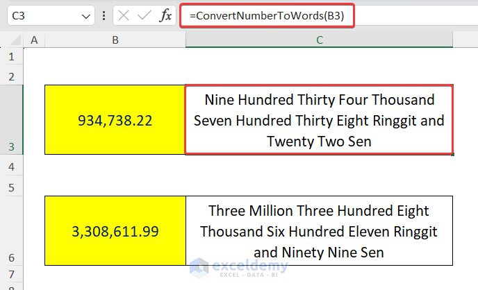
3. Now, insert the formula in Cell C3 and press Enter.
=ConvertNumberToWords(B3)I hope this code will solve your problem. If you have any other queries, please let me know in the comment section.
Regards
Mursalin,
ExcelDemy.
Hi FELIX,
Thanks for your comment. To get your desired output, you need to use the VBA code given below. We have created a custom function to convert numbers to currency words.
1. Copy the VBA code and paste it into the Module window.
2. Press Ctrl+S to save the code.
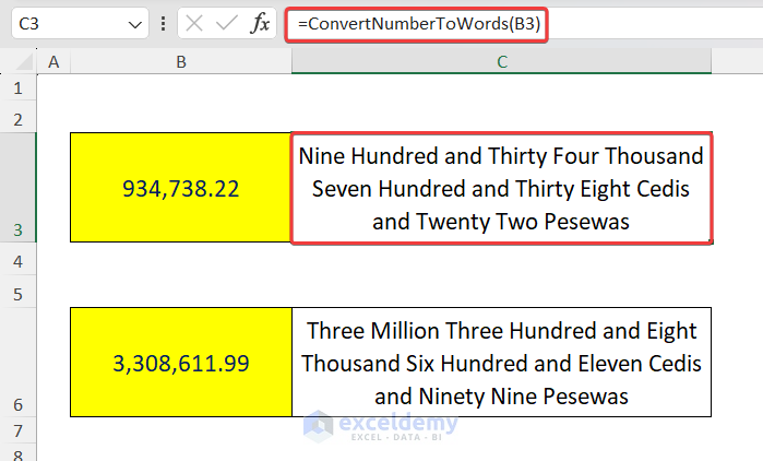
3. Now, insert the formula in Cell C3 and press Enter.
=ConvertNumberToWords(B3)I hope this code will give you the desired output. If you have any other queries, please let me know in the comment section.
Regards
Mursalin,
ExcelDemy.
Dear TAREKZHRAN,
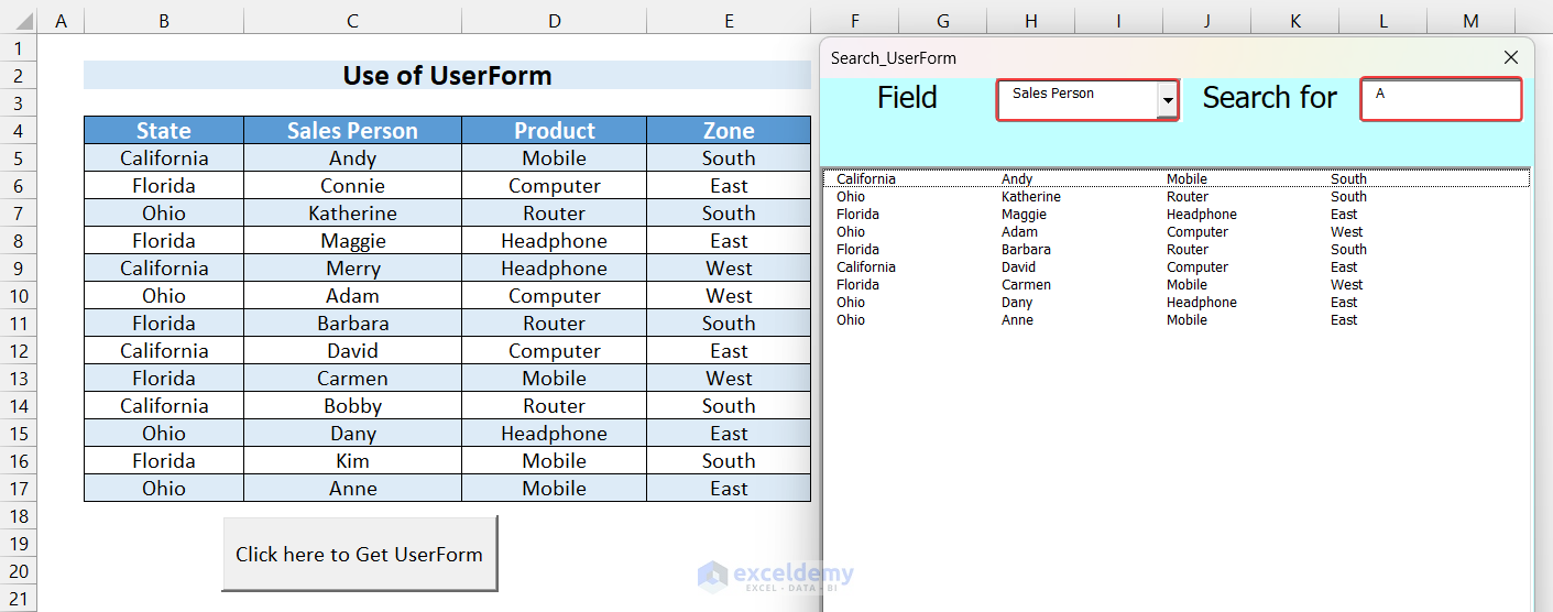
Thank you for your comment. Making a listbox of 14 columns and creating a search box will be complex. However, you can do that easily by modifying the code we provided with ComboBox.
To make a list of 14 columns change the value of col_no variable in the code we have given. Here we set 2 to 4 as col_no. Suppose your column number starts from Column B to Column O, in this case, set col_no as 2 to 15.
In the ComboBox1_Change named subprocedure change the col_header array and col_no variable like below.
Similarly, in UserForm_Initialize named sub procedure set col_no as 2 to 15 and ColumnCount to 14.
To search the alphabet from left or middle or anywhere, we will replace the Left function with the InStr function. The Left function is used to search only for the first alphabet whereas Instr will help you to find it from anywhere in the text. The modified line is below.
After modifying the code for TextBox1_Change named sub procedure will be like below.
After applying the code, you will get results like the picture below.
The Excel file of the solution is attached below. You can download and use it.
Answer.xlsm
Hope this will help you to solve your problem. Please let us know if you have other queries.
Regards,
Mursalin
ExcelDemy.
Hi INGRIDA,
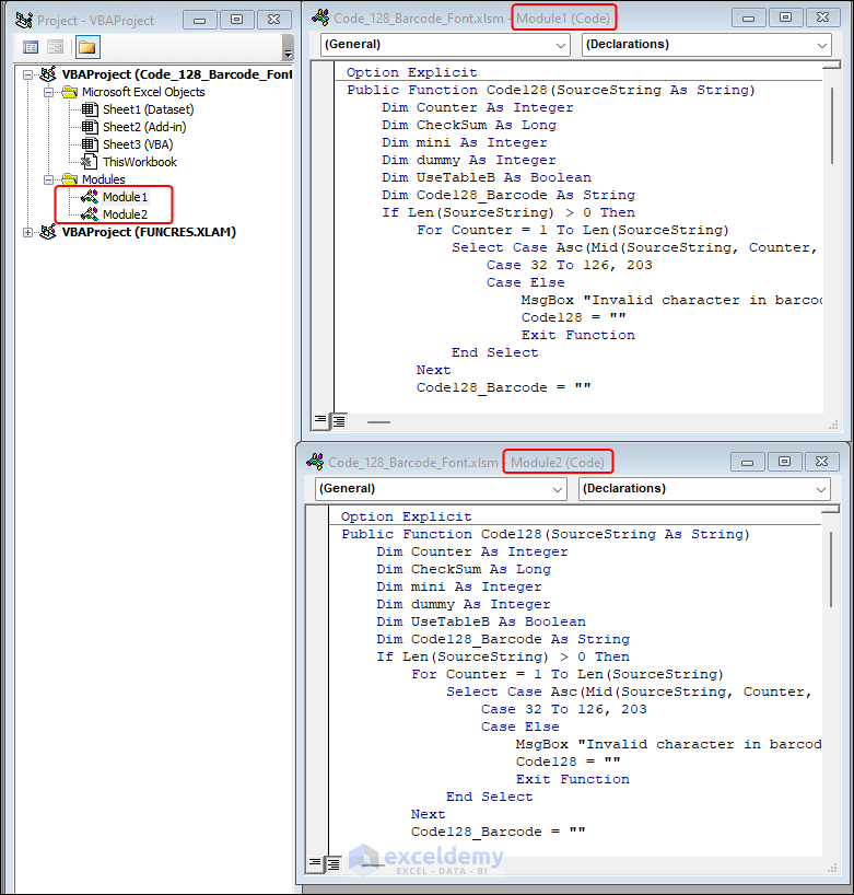
Thanks for your comment. Generally, the “Ambiguous name detected: Code128” error occurs when you insert the same formula in multiple Modules in Excel. In the picture below, you can see Module 1 and Module 2 contain the same code.
In this case, you will get the “Ambiguous name detected: Code128” error.
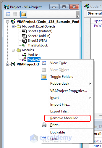
To solve it, you need to keep one module and remove others. To do so, right-click on the module you want to remove. Then, select Remove Module2.
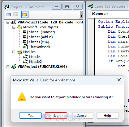
After that, select No from the pop-up message box.
After that, you can apply the “=Code128” formula without any error. I hope this will help you to solve your problem. Please let us know if you have any other queries.
Regards
Mursalin,
ExcelDemy.
Hi RINA,
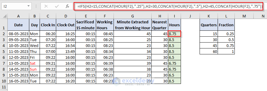
Thanks for your comment. Per your comment, we have tried implementing the conditions in our dataset. You can see the result below:
Here, we have used the formula below in Cell I2:
=IFS(H2=15,CONCAT(HOUR(F2),".25"),H2=30,CONCAT(HOUR(F2),".5"),H2=45,CONCAT(HOUR(F2),".75"))According to one of your conditions (in case of Kate), you wanted 6:23 to be displayed as 6.25. But if you want to display time to the nearest quarter on the clock, it gives 6.5. You can check out the Excel file from the link below:
Answer.xlsx
It will be easier for us to give a proper solution if you send us an Excel file with the desired outputs. You can send the Excel file to my email: [email protected]. Please let us know if you have any other queries.
Regards
Mursalin,
Exceldemy.
Dear LYDETH,
Thanks for your comment. In this article, we have shown how to copy exact formulas in Excel both using cell reference and without using cell reference. So, you can use not only methods 12 and 13 but also methods 4, 6, 7, 8, 9, and 10 for copying the exact formulas. And if you want to copy the exact formula with relative cell address you can follow methods 1, 2, 3, 5, and 11.
Please let us know if you have any other queries.
Regards
Mursalin,
Exceldemy.
Dear SARAH,
Thanks for your comment. The Variance Inflation Factor (VIF) measures the degree of multicollinearity in a set of explanatory variables in a regression model. VIF values greater than 1 indicate that the explanatory variables are correlated to some degree. However, a VIF value of infinity is not an indication of perfect correlation.
When the R-squared value is equal to 1, it indicates that the regression model perfectly fits the data. But, setting the R-squared value to 1 does not make sense in practice as it implies that the model explains all the variation in the data, which is usually not the case.
If the R-squared value is set to 1, the VIF becomes undefined rather than infinity. This is because the formula for VIF involves dividing by the difference between 1 and the R-squared value, and division by zero is undefined.
So we can say, a large VIF value indicates some degree of correlation between the explanatory variables, but an infinite VIF does not necessarily indicate perfect correlation. Setting the R-squared value to 1 makes the VIF undefined rather than infinity.
I hope this answer will help to interpret a VIF where the R-square is 1. Please let us know if you have any other queries.
Regards,
Mursalin,
Exceldemy.
Hi KIM,
Thanks for your comment. To explain the step-by-step solution, we used the following question here.
“Suppose, a machine is used to produce two interchangeable products. The daily capacity of the machine can produce at most 20 units of product 1 and 10 units of product 2. Alternatively, the machine can be adjusted to produce at most 12 units of product 1 and 25 units of product 2 daily. Market analysis shows that the maximum daily demand for the two products combined is 35 units. Given that the unit profits for the two respective products are $10 and $12, which of the two machine settings should be selected?”
This question is also stated before starting STEP 1.
Analyzing the above question, we can find the following constraints:
Constraint 1:
X1+X2<=35
Because the maximum daily demand for the two products combined is 35 units.
Here, X1 is the quantity of Product 1 and X2 is the quantity of Product 2.
Constraint 2:
X1-8Y<=12
This constraint is for Product 1. In this constraint, we have combined the conditions for both settings for Product 1. In setting 1, product 1 can be produced at most 20 units; in setting 2, product 2 can be produced at most 12 units.
Here, Y denotes which setting is selected. If setting 1 is selected, then Y will be 1 and if setting 2 is selected, then Y will be 0.
For example, if setting 1 is selected, then we can set Y=1. So, the equation will be:
X1-8.1<=12
As a result, the simplified constraint will be X1<=20 which clearly states the condition for product 1 stated in the first setting.
Constraint 3:
X2+15Y<=25
This constraint is for Product 2. In this constraint, we have combined the conditions for both settings for Product 2. In setting 1, product 2 can be produced at most 10 units; in setting 2, product 2 can be produced at most 25 units.
Here, Y denotes which setting is selected. If setting 1 is selected, then Y will be 1 and if setting 2 is selected, then Y will be 0.
For example, if setting 1 is selected, then we can set Y=1. So, the equation will be:
X2+15.1<=25
As a result, the simplified constraint will be X2<=10 which clearly states the condition for product 2 stated in the first setting.
Constraint 4:
Y={0,1}
The value of Y will be 0 or 1. 1 represents the selection of setting 1 and 0 represents the selection of setting 2.
Non–Negative restriction:
X1,X2>=0
The quantity of the products can not be negative.
Constraints 1, 2 & 3 are the main constraints here.
In the Mixed Integer Linear Programming part, we have used a set of conditions as constraints where X1, X2, and X3 are integers and Y1, Y2, and Y3 are binary numbers.
I hope this explanation of the constraints will help you. Please let me know if you have any queries.
Regards
Mursalin,
Exceldemy.
Hi MYLES,
Thanks for your comment. We are very glad to know that we could be of help to you. Let us know if you have any queries.
Good luck.
Hi FREEJOJOEY,
Sorry to hear about your problem. I am replying to you on behalf of Exceldemy. The Developer tab is not included in the ribbon by default. But you can easily add it. To add the Developer tab, please the steps of the link below:
Get Developer Tab
After inserting the Developer tab, follow the steps of the article. If you follow the steps correctly, you will get the scannable barcodes. You must insert the VBA using the Developer tab as stated in STEP 2 for getting the correct characters.
Thanks!
Hi STEPHEN,
Thanks for reaching out to us. I am replying to you on behalf of Exceldemy. We will be happy to help you.
Please send the Excel file to [email protected]. Also, mention what you want to update in the Excel file. We will try to give the solution as early as possible.
Thanks!
Hi KIERAN,
Thanks for your comment. This is Mursalin from Exceldemy. I am not quite sure why you are getting a barcode that is not scannable. Because in my case, after changing the text to Code 128, I am getting the desired scannable barcode.
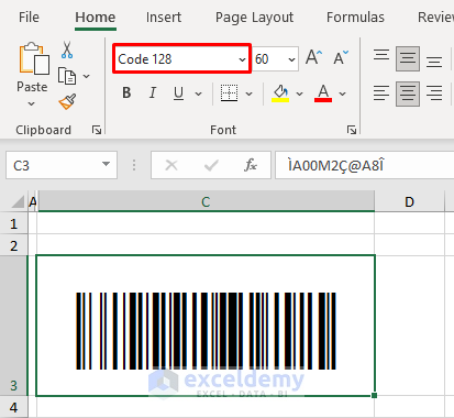
It will be helpful for me if you provide the Excel file or an image in the comment section. Or you can send the Excel file to [email protected]. I hope I can give a solution after watching the file.
Thanks!
Hi KATIA,
Thanks for your comment. I am replying to you on behalf of Exceldemy. To find the average, you can use the AVERAGE function. For Method 1, you can follow the steps below.
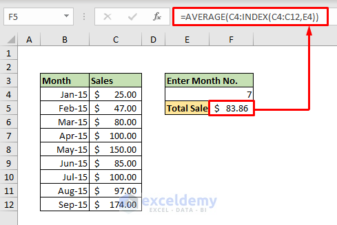
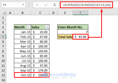
STEPS:
1. Firstly, select Cell F5 and type the formula below:
=AVERAGE(C4:INDEX(C4:C12,E4))2. Press Enter to see the result.
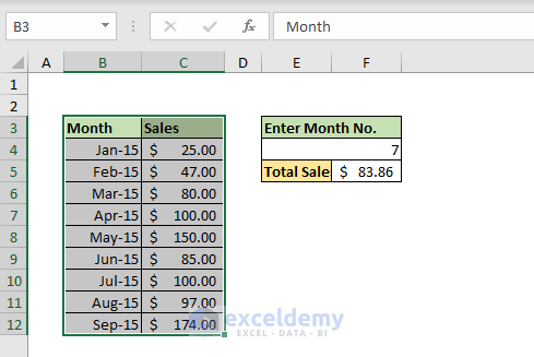
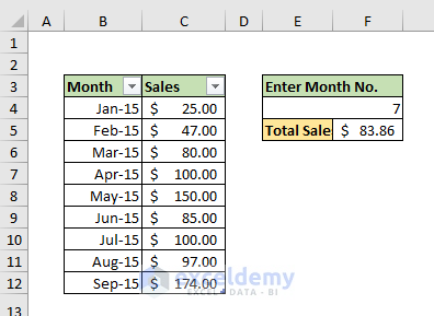
3. Secondly, select the range B3:C12.
4. Press Ctrl + T to convert the range into a table.
5. A message box will appear.
6. Click OK to proceed.
7. As a result, you will see a table like the picture below.
8. Now, if you add Oct-15 in Cell B13, then the table and formula of Cell F5 will automatically update.
For Method 2, you can follow the above steps and use the formula below:
=AVERAGE(OFFSET(B4,0,0,1,-MONTH(B3)):B4)For Method 3, use the formula below and convert the range into a table:
=AVERAGEIFS(C4:C17, B4:B17, ">="&B4, B4:B17, "<="&F5)You can also find the formulas in the workbook below:
Workbook with AVERAGE Formulas.xlsx
I hope this will help you to solve your problems. Please let us know if you have other queries.
Thanks!
Hi BEN,
Thanks for your comment. I am replying to you on behalf of Exceldemy. To know more about copying formulas across cells, you can check the link below.
Copy Formulas Across Cells
Thanks!
Hi JESSICA,
Thanks for your comment. I am replying to you on behalf of Exceldemy. You can check the comment thread for the answer. Also, to know more about copying formulas across cells, you can check the link below.
Copy Formulas Across Cells
Thanks!
Hi ROBYN,
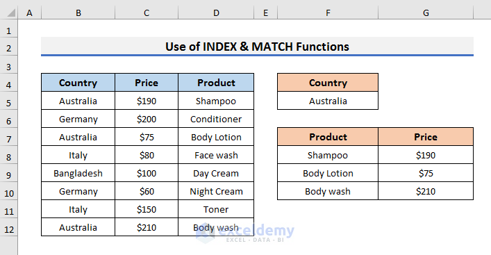
Thanks for your comment. I am replying to you on behalf of Exceldemy. To get the results across the cells, you need to drag the Fill Handle to the right side and make the necessary changes if needed. Suppose, we also need the Price along with the products. We can get the prices using some steps. Let me show you the process in the steps below.
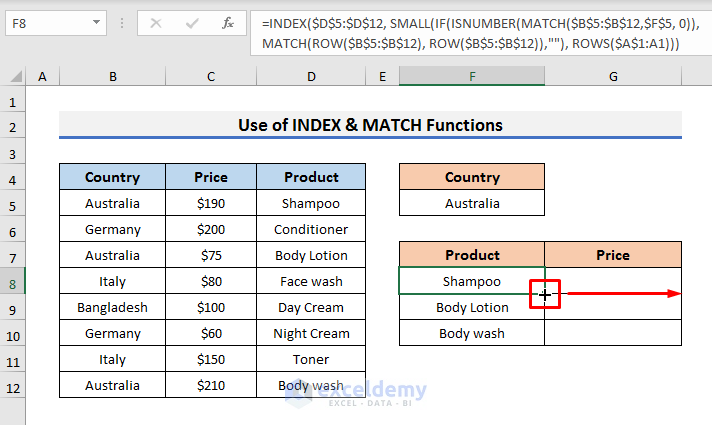
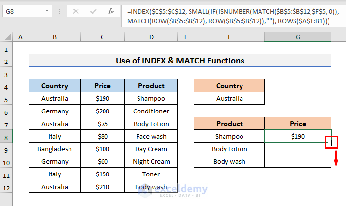
STEPS:
1. Firstly, put the cursor on the bottom corner of Cell F8. It will turn into a small plus sign.
2. Now, drag the Fill Handle to the right to Cell G8.
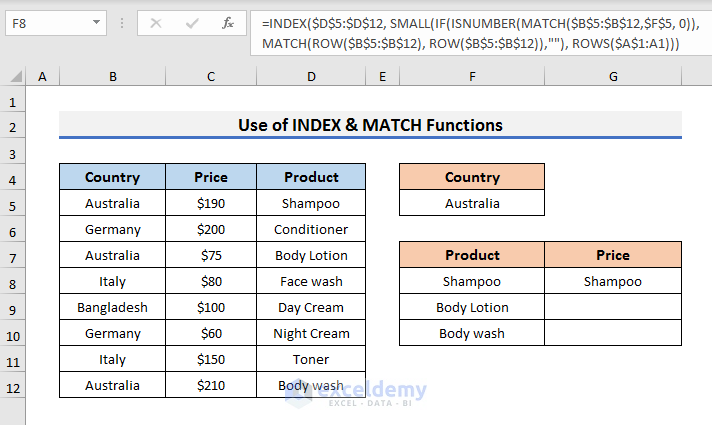
3. It will show the same result and formula because the range D5:D12 is locked.
4. Now, select Cell G8 and go to the Formula Bar.
5. Type
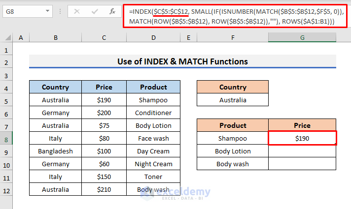
$C$5:$C$12in place of$D$5:$D$12because Column C contains the prices.6. Press Enter.
7. After that, drag the Fill Handle down.
8. Finally, you will see the prices of the products.
To know more about copying formulas across cells you can check the article below.
Copy Formula Across Cells
I hope this will help you to solve your problem. Please let us know if you have other queries.
Thanks!
Hi JOJO,
Thanks for your comment. I am replying to you on behalf of Exceldemy. You can use VBA to remove texts that have strikethrough in them. Suppose, you have some text strings like the picture below:
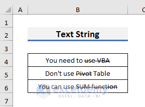
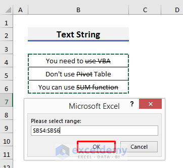
Let’s follow the steps below to remove the texts with a strikethrough.
STEPS:
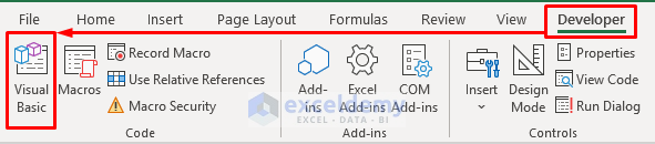
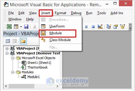
1. Firstly, go to the Developer tab and click on the Visual Basic option.
2. Secondly, select Insert >> Module to open the Module window.
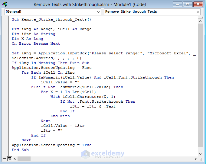
3. Now, copy the code below and paste it into the Module window:
Sub Remove_Strike_through_Texts()Dim iRng As Range, iCell As RangeDim iStr As StringDim X As LongOn Error Resume NextSet iRng = Application.InputBox("Please select range:", "Microsoft Excel", _Selection.Address, , , , , 8)If iRng Is Nothing Then Exit SubApplication.ScreenUpdating = FaseFor Each iCell In iRngIf IsNumeric(iCell.Value) And iCell.Font.Strikethrough TheniCell.Value = ""ElseIf Not IsNumeric(iCell.Value) ThenFor X = 1 To Len(iCell)With iCell.Characters(X, 1)If Not .Font.Strikethrough TheniStr = iStr & .TextEnd IfEnd WithNextiCell.Value = iStriStr = ""End IfNextApplication.ScreenUpdating = TrueEnd Sub4. Press Ctrl + S to save the code.
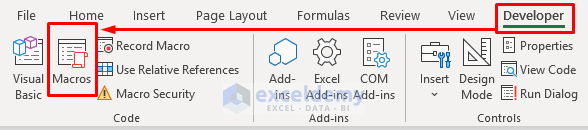
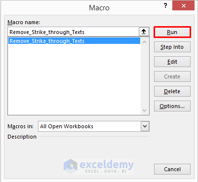
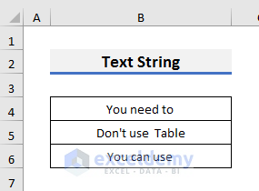
5. After that, go to the Developer tab and select Macros.
6. In the Macro window, select the desired code and Run it.
7. A message box will appear.
8. Select the range from where you want to remove the strikethrough texts.
9. Finally, click OK to proceed.
10. As a result, the texts with strikethrough will be removed.
I hope this will help you to solve your problem. Please let us know if you have other queries.
Thanks!
Hi CHRIS,
Thanks for your comment. I am replying to you on behalf of Exceldemy. We can use VBA to loop through rows of data and extract the desired data.
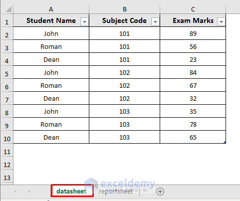
For example, we will use a VBA to look for the marks of a specific student in the datasheet, copy them and paste the marks into the reportsheet. You can see the marks of all students in the picture below:
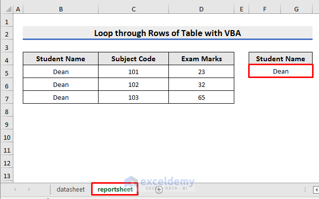
We will copy the marks of a specific student and paste them into the reportsheet.
For that purpose, you can use the code below:
Sub Loop_Through_and_Extract_Data()Dim datasheet As Worksheet 'From where data will be copiedDim reportsheet As Worksheet 'where data will be pastedDim StudentName As StringDim finalrow As IntegerDim i As Integer 'row counter'set variablesSet datasheet = Sheet1Set reportsheet = Sheet3StudentName = reportsheet.Range("F5").Value 'Cell F5 of reportsheet contains the student name'clear old datareportsheet.Range("B5:D200").ClearContents'go to datasheet and start searching and copyingdatasheet.Selectfinalrow = Cells(Rows.Count, 1).End(xlUp).Row'loop through rows to find matching recordsFor i = 2 To finalrowIf Cells(i, 1) = StudentName Then 'if the name matches, then copyRange(Cells(i, 1), Cells(i, 3)).Copy 'copy columns 1 to 3 (A to C)reportsheet.Select 'go to reportsheetRange("B200").End(xlUp).Offset(1, 0).PasteSpecial xlPasteAll 'paste values in the reportsheetdatasheet.Select 'go back to datasheet and continue searchingEnd IfNext ireportsheet.SelectRange("A1").SelectEnd SubI have also attached the Excel file below:
Loop Through Rows.xlsm
I hope this will help to solve your problem. Please let us know if you have other queries.
Thanks!
Hi DAWID,
Thanks for your comment. Sorry to hear that you are not getting the desired output. I have tried to convert 192697 and 194898 to barcodes using the same code. In my case, it worked. You can see the result below:
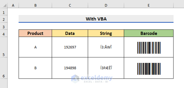
I am also attaching the Excel file below:
Answer.xlsm
Moreover, the VBA code is not error-free. It can introduce errors sometimes. You can copy the code and paste it into a new workbook. It may help you to get the desired results.
I hope this will help you to solve your problem. Please let us know if you have other queries.
Thanks!
Hi AHMETCAN,
Thanks for your comment. I am replying to you on behalf of Exceldemy. To get all the desired values from the list, you need to drag the Fill Handle down to copy the formula. You can follow the steps below to get all the values.
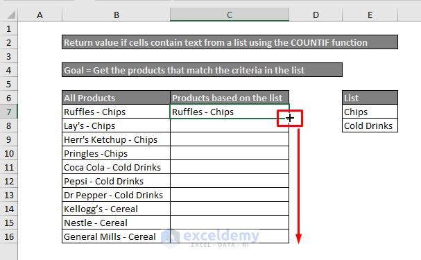
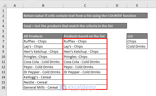
STEPS:
1. Firstly, select Cell C7 and type the formula below:
=IF(OR(COUNTIF(B7,"*"&$E$7:$E$8&"*")),B7,"")2. Press Enter to see the result.
3. Thirdly, move the cursor to the bottom right corner of Cell C7, it will turn into a small black plus sign.
4. Now, drag the Fill Handle down to Cell C16.
5. Finally, you will see results like the picture below.
I hope this will help you to solve your problems. Please let us know if you have other queries.
Thanks!
Hi MIKE M,
Sorry for the late reply. I am replying to you on behalf of Exceldemy. You can mail your problem to [email protected]. Our team will take a look and try to give a solution to your problem.
Thanks!
Hi KARTHIKA,
Thanks for your comment. To insert checkboxes without shortcuts, you can follow the steps below:
STEPS:
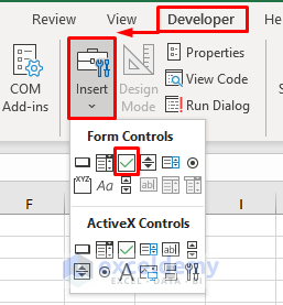
1. Go to the Developer tab and click on the Insert option.
2. A drop-down menu will appear.
3. You can select the checkbox from the “Form Controls” section.
If you don’t find the Developer tab in the ribbon, then you need to add it from the Customize the Ribbon option. You will find the detail in the link below:
https://www.exceldemy.com/add-a-checkbox-in-excel/#2_Steps_to_Add_a_Checkbox_in_Excel
I hope this will help you to solve your problem. Please let us know if you have any other queries.
Thanks!
Hi PETE,
Thanks for your comment. I am replying on behalf of Exceldemy. To paste the values, you can try the code below:
Sub Copy_Data_from_Another_Workbook()Dim wb As WorkbookDim newwb As WorkbookDim rn1 As RangeDim rn2 As RangeSet wb = Application.ActiveWorkbookWith Application.FileDialog(msoFileDialogOpen).Filters.Clear.Filters.Add "Excel 2007-13", "*.xlsx; *.xlsm; *.xlsa".AllowMultiSelect = False.ShowIf .SelectedItems.Count > 0 ThenApplication.Workbooks.Open .SelectedItems(1)Set newwb = Application.ActiveWorkbookSet rn1 = Application.InputBox(prompt:="Select Data Range", Default:="A1", Type:=8)wb.ActivateSet rn2 = Application.InputBox(prompt:="Select Destination Range", Default:="A1", Type:=8)rn1.Copyrn2.PasteSpecial xlPasteValuesnewwb.Close FalseEnd IfEnd WithEnd SubHere, we have used the code of Method 1. We changed the highlighted lines to copy and paste only the values.
I hope this will help you solve your problem. Please let us know if you have any other queries.
Thanks!
Hi EVAGGELOS,
Thanks for your comment. I am replying on behalf of Exceldemy. Unfortunately, you can’t stop the update at a given time. But you can stop it instantly using a slightly different code and keyboard shortcut. You can follow the steps below for that purpose.
STEPS:
1. Copy and Paste the code in the Module window:
Public RunWhen As DoubleSub UpdateCell()RunWhen = Now + TimeValue("00:00:05")Application.OnTime RunWhen, "UpdateCell"Application.CalculateEnd SubSub StopUpdate()On Error Resume NextApplication.OnTime RunWhen, "UpdateCell", , FalseEnd Sub2. Press Ctrl + S to save it.
3. Now, press Alt + F8 to open the Macro window.
4. Select StopUpdate from there and then, click on Options. It will open the Macro Options box.
6. In the Macro Options box, type K in the “Shortcut Key” field.
7. Then, click OK to proceed.
8. Now, run the UpdateCell code.
9. To stop updating, press Ctrl + K and the update will be stopped.
I hope this will help you solve your problem. Please let us know if you have any other queries.
Thanks!
Hi A V S S PRASAD,
Sorry for the late reply. I am replying to you on behalf of Exceldemy. To match the addresses, you need to use the INDEX-MATCH functions. You will find similar formulas in the articles below.
https://www.exceldemy.com/index-match-multiple-criteria-partial-text/
https://www.exceldemy.com/index-match-partial-match/
I hope this will help you to solve your problem.
Thanks!
Hi TONY O’BRIEN,
Sorry for the late reply. I am replying to you on behalf of Exceldemy. To get multiple companies, you can use the formula below in Cell G13:
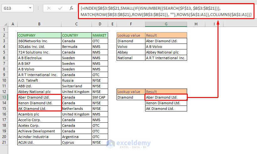
=INDEX($B$3:$B$21,SMALL(IF(ISNUMBER((SEARCH($F$13,$B$3:$B$21))),MATCH(ROW($B$3:$B$21),ROW($B$3:$B$21)), ""),ROWS($A$1:A1)),COLUMNS($A$1:A1))Remember, it is an array formula. You can follow the steps below to get the results.
1. Firstly, type Diamond in Cell F13.
2. Secondly, type the above formula in Cell G13.
3. Press Ctrl + Shift + Enter together.
4. After that, drag the Fill Handle down to get all 3 values.
For more information, you can check the article below.
https://www.exceldemy.com/index-match-multiple-criteria-partial-text/
I hope this will help you to solve your problem.
Thanks!
Hi BRIAN WINKLE,
Sorry for the late reply. I am replying to you on behalf of Exceldemy. To create a timestamp like the given example, you can take a look at the article below.
https://www.exceldemy.com/create-a-timesheet-in-excel/
I hope this will help you to solve your problem.
Thanks!
Hi JIM,
Sorry for the late reply. I am replying to you on behalf of Exceldemy. You need to apply the formula below in Cell G16:
=24-((C16-F16)-(D16-E16))*24I hope this will help you to solve your problem. Please let us know if you have other queries.
Thanks!
Hi JOE FRAZIER,
Thanks for your comment. I am replying to you on behalf of Exceldemy. In this article, Cells I16:I22 of Column I counts the overtime for each day of a week. That means if you want to see the overtime for Monday, you need to check Cell I16. So, you can use the same formula to calculate overtime for a single day.
I hope this will help you to solve your problem. Please let us know if you have other queries.
Thanks!
Hi FEITY LAU,
Sorry for the late reply. I am replying to you on behalf of Exceldemy. I guess you are facing the problem because of not defining the names. Here, Cell D12 is renamed as work_hours_per_week. You can use the Name Manager in the Formulas tab to define the name. To check the defined names, follow the steps below.
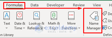
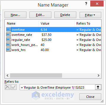
Firstly, download the practice book, go to the Formulas tab and select Name Manager.
In the Name Manager box, you will find all the defined names.
To apply the same formula in your new spreadsheet, you need to define the names using the Name Manager. To do that, you can follow the link below.
https://www.exceldemy.com/excel-edit-named-range/
Thanks!
Hi DEE ZELAYA,
Sorry for the late reply. I am replying to you on behalf of Exceldemy. Here, Cell D12 is renamed as work_hours_per_week. You can use the Name Manager in the Formulas tab to define the name. To check the defined names, follow the steps below.


Firstly, download the practice book, go to the Formulas tab and select Name Manager.
In the Name Manager box, you will find all the defined names.
To apply the same formula in your new spreadsheet, you need to define the names using the Name Manager. To do that, you can follow the link below.
https://www.exceldemy.com/excel-edit-named-range/
Thanks!
Hi CHRISTIAN,
Thanks for your comment. I am replying to you on behalf of Exceldemy. The time difference in the above article is in Number format. That is why 8.17 doesn’t mean 8 hours 17 min. It actually means 8 hours and 10 minutes. To get the results in the desired format, you can follow the steps below.
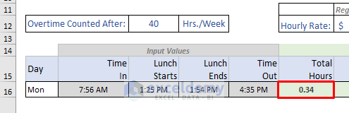
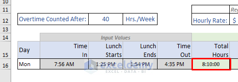
First of all, select Cell G16 in the dataset and type the formula below:
=((F16-C16)-(E16-D16))Hit Enter to see the result.
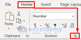
Select Cell G16 again, go to the Home tab, and click on the Number Format icon. It will open the Format Cells window.
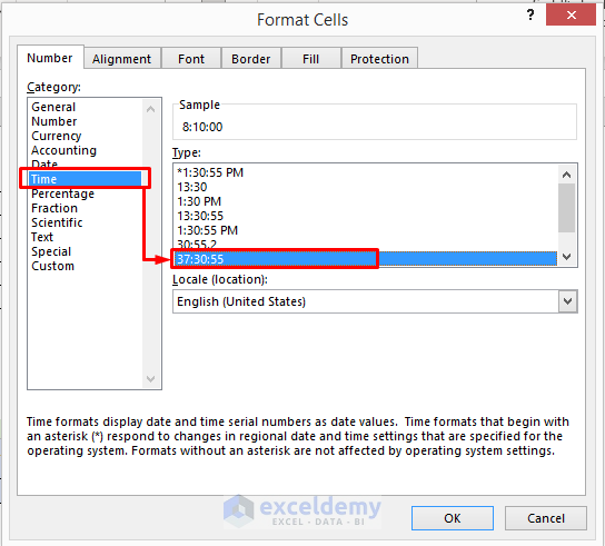
In the Format Cells window, click on the Number tab and select Time.
Then, select 37:30:55 from the Type box.
As a result, you will see the result in the desired format.
I hope this will solve your problem. Please let us know if you have any other queries.
Thanks!
Dear JESSE BATES,
Thanks for your comment. Declaring variable types is not mandatory in VBA. VBA by default assigns the necessary data type to any variable, you just need to put the values. In the given code, the timer variable contains the data type Double.
Please let us know if you have any other queries.
Thanks!
Dear AG,
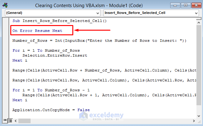
Thanks for your comment. To avoid the Run time error in VBA, you need to add an error handling line inside the code. There are different error-handling commands in VBA. To solve the problem, add the below line after the Sub procedure.
On Error Resume Next
You need to add the above line inside the code like the picture below.
To know more about handling errors in Excel VBA, you can check out the article below.
https://www.exceldemy.com/excel-vba-on-error-resume-next/
I hope this reply will solve your problem. Please let us know if you have any other queries.
Thanks!
Dear MICHAEL,
Thanks for your comment. You can insert a Tab using “~009” inside the string. For example, XXXX.1TAB123456 can be written as XXXX.1~009123456. But unfortunately, it will not show two separate fields in one barcode. From my understanding, you need to use other barcode fonts for that purpose.
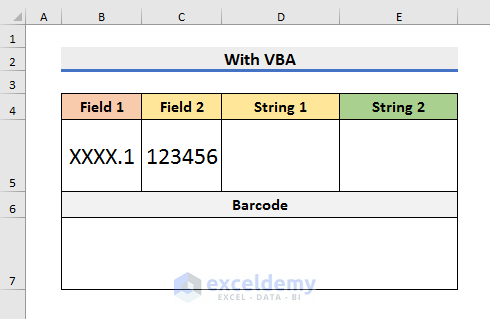
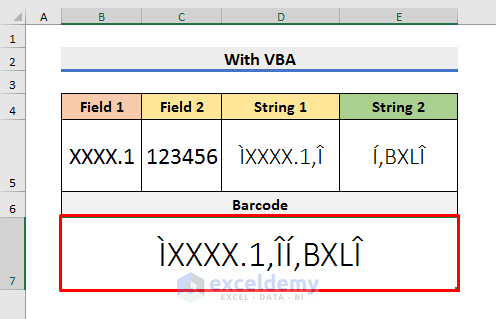
Otherwise, you can look at the solution below. But this solution will not provide you with one barcode. Here, we tried to concatenate two separate barcodes in one cell. Here, we will use the dataset below.
Let’s follow the steps below for the solution.
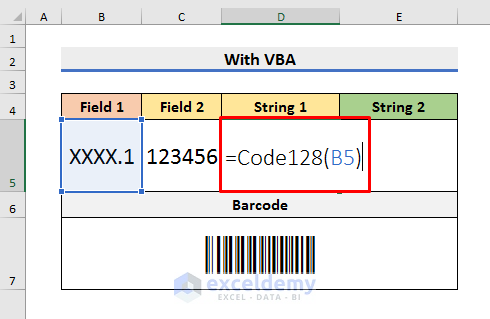
● Firstly, change the fields into barcode strings.
● To do so, select Cell D5 and type the formula below:
=Code128(B5)
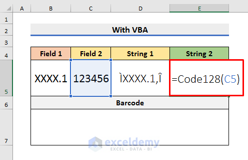
● Also, do the same for the second field.
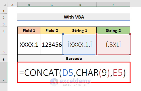
● After that, select Cell B7 and type the formula below:
=CONCAT(D5,CHAR(9),E5)
● Hit Enter to see the result.
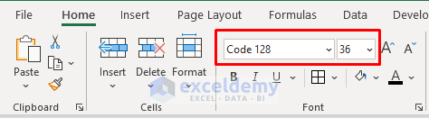
● Now, select Cell B7 again and change the font theme to Code 128.
● Also, adjust the font size.
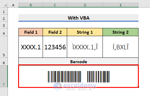
● Finally, you will get results like the picture below.
I hope this solution will help benefit you to some extent. Please let us know if you face any other issues.
Thanks!
Hello CRISNA,
Thanks for your comment. You can’t generate the text below the barcode with the code 128 font we used here. But you can use the Libre Barcode 128 Text font for that. Also, you can follow this article https://www.exceldemy.com/generate-barcode-numbers-in-excel/ to generate characters below the barcode. I hope this will help you to solve your problem. Please let us know your queries if you face any issues.
Thanks.
Hi MKM,
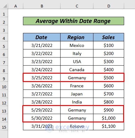
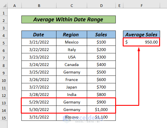
Thanks for your comment. To answer your question, we can use the dataset below. It contains 3 rows of sales for Germany. The first sale happened in March and the other two sales happened in May. From this dataset, we can easily calculate the average sales for May in Germany.
To calculate the average sales for May in Germany, select Cell F5 and type the formula below:
=AVERAGEIFS(D5:D15, B5:B15,”<=5/31/2022", B5:B15,">=5/01/2022″,C5:C15,”Germany”)
Press Enter to see the result.
I hope this will help you to solve your problem. Please let us know your queries if you face any issues.
Thanks.
Dear NEIL,
Thanks for your comment. Code 128 barcode font has 106 unique representations and supports standard ASCII characters. Unfortunately, Õ and Œ – these two characters are not supported by code 128 barcode font. But you can try other barcode fonts to solve this issue. You can use the free online barcode generator for that purpose. I hope this will help you to solve your problem.
Thanks.
Dear CHRIS,
Thanks for your comment. Excel omits the leading zero by default. So, it’s not possible to get the desired barcode.
• To solve this, you must add an apostrophe (‘) in front of the leading zero.
• So, select Cell C5 in the VBA sheet of the workbook.
• Type ‘02628107336750 in Cell C5.
• Press Enter.
• You will get your results in Cell D5.
I hope this will help you to solve your problem.
Thanks.
Hello, Abu!
Thanks for your comment. Unfortunately, it is not possible to show the expected end date dynamically after each pre-payment. Because the dataset changes dynamically after a pre-payment. But you can find the expected payment date after each month using the formula below. For the dataset, we have used in this article, you can type the formula in Cell H8:
=DATE(YEAR(H7),MONTH(H7)+(12/$J$15),DAY(H7))
Here, Cell H7 contains the loan starting date and Cell J15 contains the number of yearly payments.
You can also take a look at this article https://www.exceldemy.com/student-loan-payoff-calculator-with-amortization-table-excel/ for an explanation of the formula. I hope this will help you to solve your problem.
Thanks!
Hello, Dom!
Thanks for your feedback. If you are facing any problems generating code 128 barcode font in Excel, then you can ask here. We will try to reply to you as soon as possible.
Thanks!
Hello, Bimen!
Sorry to hear that you are facing problems converting minutes to decimal numbers. You can send your excel file to [email protected] and we will try to give a solution to your problem.
Thanks!
Hi BIPLAB,
Thanks for your query. You can build a formula with the nested CONCAT function. In that case, you don’t need any helper column. For the dataset we have discussed in the article, the formula will be:
=CONCAT(CONCAT(B5,” “,C5,” “,D5),”,”, CONCAT(B6,” “,C6,” “,D6),”,”,CONCAT(B7,” “,C7,” “,D7),”,”,CONCAT(B8,” “,C8,” “,D8))
You can also use the VBA code below. To apply this, you need to select the rows of the first column of the dataset and then run the code from the Macro window.
Sub Merge_Rows_with_Comma()
Dim iSelection As Range
Dim iRow As Range
Dim iCell As Range
Dim iStr As String
Application.ScreenUpdating = False
On Error Resume Next
Set iSelection = Intersect(Selection, ActiveSheet.UsedRange)
For Each iRow In iSelection.Rows
For Each iCell In iRow.Cells
iStr = iStr & ” ” & VBA.Trim$(iCell)
Next iCell
iRow.ClearContents
iRow.Cells(1, 1).NumberFormat = “@”
iRow.Cells(1, 1) = Mid(iStr, 2)
iStr = vbNullString
Next iRow
For Each iCell In iSelection
iStr = iStr & “,” & VBA.Trim$(iCell)
Next
With ActiveWindow
.Selection.ClearContents
.Selection(1, 1).NumberFormat = “@”
.Selection(1, 1).Value = Mid(iStr, 2)
End With
End Sub