Using the INDEX-MATCH Function with Multiple Criteria for a Partial Text in Excel – 2 Methods

Excel INDEX Function Introduction

The INDEX function returns the value of a cell at the intersection of a row and column in an array or range.

• Syntax

INDEX (array, row_num, [col_num], [area_num])

• Arguments

array: It is the first compulsory argument: the constant array or the cell range.

row_num: It is the second compulsory argument: the row number in the array.

[col_num]: This is an optional argument: the column number in the array.

[area_num]: It is also an optional argument:  it selects a range in a reference and returns the intersection of row_num and col_num.

Excel MATCH Function Introduction

The MATCH function looks for a specific value in an array or range and returns its relative position.

• Syntax

MATCH (lookup_value, lookup_array, [match_type])

• Arguments

lookup_value: This is the first compulsory argument: It is the value searched in a range or array.

lookup_array: It is the second compulsory argument. It is the array.

[match_type]: It is an optional argument: the type of match. For an exact match, use 0. Use 1 and -1. 1 to get the greatest value less than or equal to the lookup_value and -1 to get the smallest value greater than or equal to the lookup_value.

Method 1 – Using the Excel INDEX-MATCH Formula with Multiple Criteria for a Partial Text

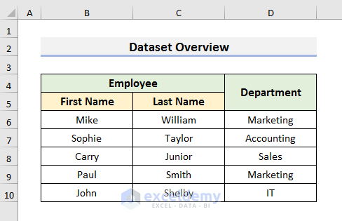
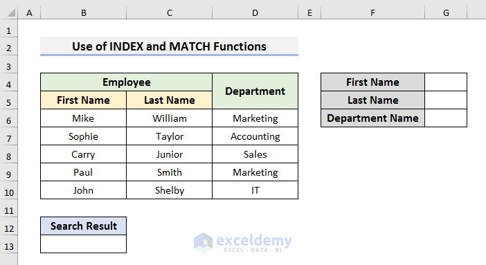
The dataset  contains the First Name, Last Name, and the Department of employees. To return a result based on partial text:

STEPS:

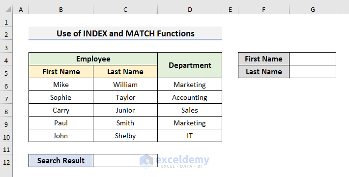
• Create cells to insert the partial texts and display the Search Result. Here,  G4 and G5.

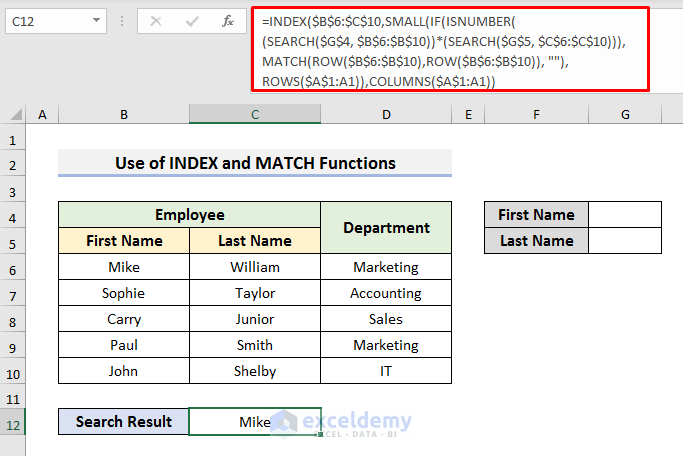
• Select C12 and enter the formula:

• Press Enter.

 Formula Breakdown

• Drag the Fill Handle to the right.

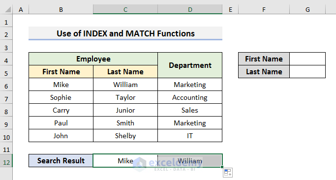
The Search Result is Mike William (no partial text  was entered in G4 and G5).

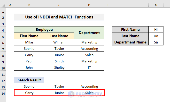
• Enter the partial text in G4 and G5. Here,  “So” in G4 and “Ta” in G5.
• Sophie Taylor is the Search Result.

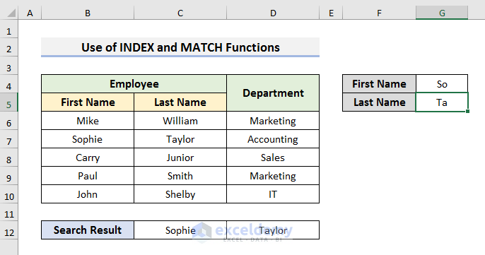
The formula searches “So” in the First Name column and then, “Ta” in the Last Name column. As it found a match, it displays the result.

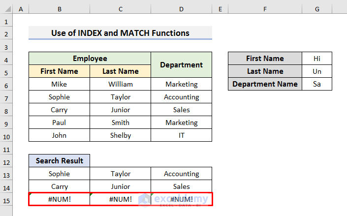
• If you change the partial text of the Last Name, it will display #NUM.

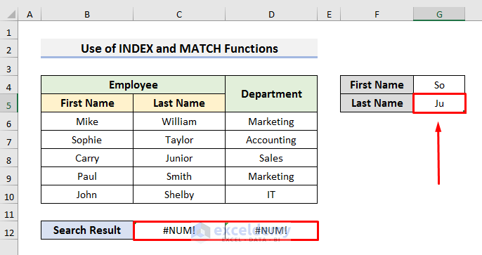
It finds a match in the First Name column, but the partial text of the Last Name does not match the value found in the First Name column.

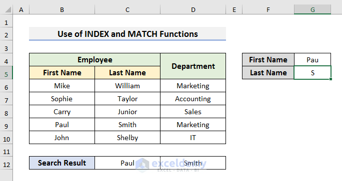
• If you change the partial texts, the value will be updated.

Method 2 – Applying the INDEX-MATCH Formula with Multiple Criteria for a Partial Text to Get Multiple Records

Use the INDEX and the MATCH functions with multiple criteria for a partial text to get multiple records.

To see the full name of the employee and his/her department in the search result:

STEPS:

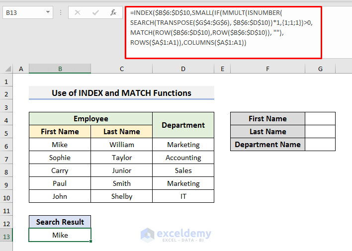
• Select B13 and use the formula:

• Press Enter.

Formula Breakdown

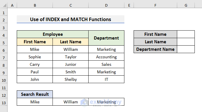
• Drag the Fill Handle to the left to D13. You will see Mike’s full name and department (there are no partial texts in G4 to G6).

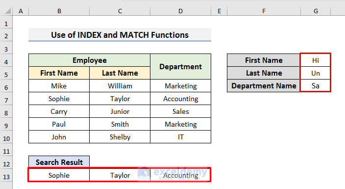
• Enter the partial texts in G4:G6.
• The Search Result will automatically be updated.

• Select  B13:D13.
• Drag the Fill Handle down to Row 14.

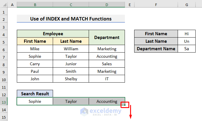
• You will see Carry’s full name and department because it matches the partial text of theLast Name .

• Use the Fill Handle. It will display #NUM as no more matches are found.

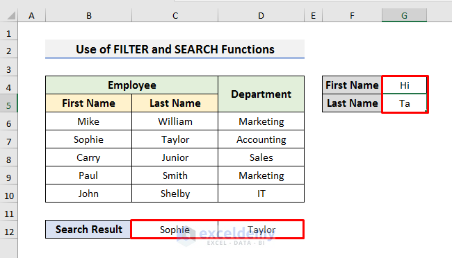
Use The FILTER & SEARCH Functions with Multiple Criteria for a Partial Text in Excel

Use the FILTER and SEARCH Functions. This is the same dataset and structure used in Method 1.

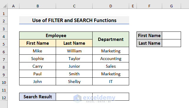
STEPS:

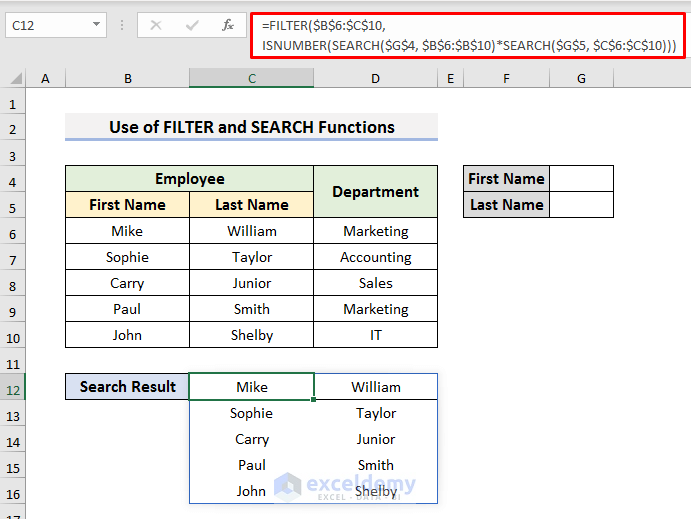
• Select C12 and enter the formula:

• Press Enter to see the result.
• You will see the whole dataset as there is no partial text.

Formula Breakdown

• Enter “Hi” in G4 and “Ta” in G5.
• Press Enter to see an automatic update in the Search Result.

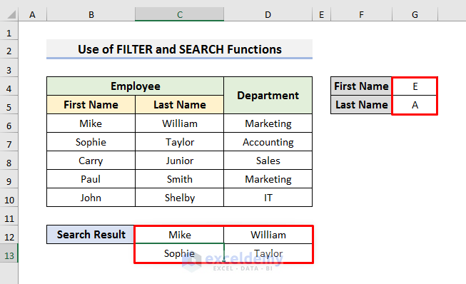
• If you change the partial texts, it will display all values containing the partial text.

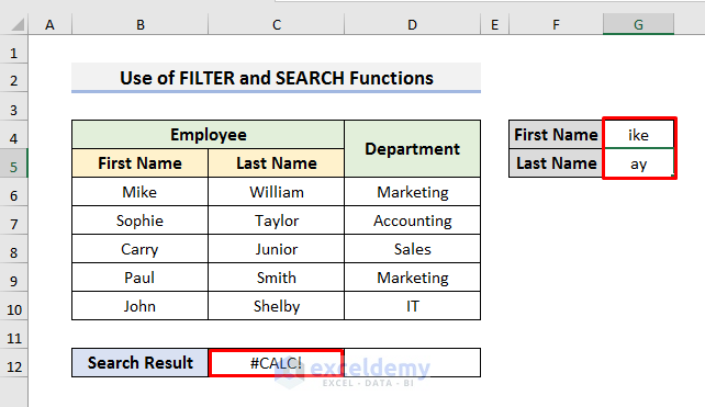
• If it does not find a match, it will display #CALC.

Download Practice Book

Download the practice book here.

<< Go Back to Partial Match Excel | Formula List | Learn Excel