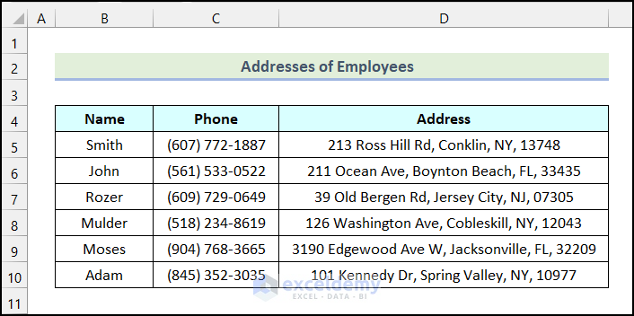
The sample dataset showcases the Addresses of Employees in a company.
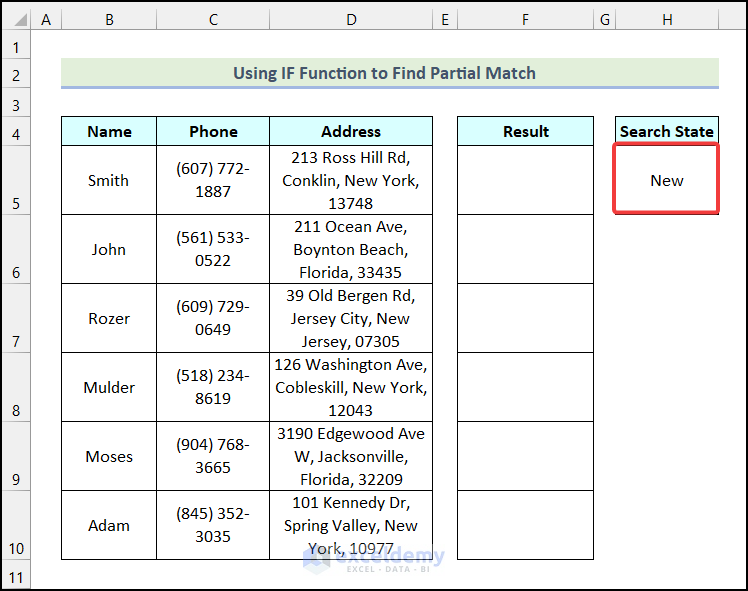
To check whether a a partial match for a given state name is in the Address column, enter “New” in the Search State column
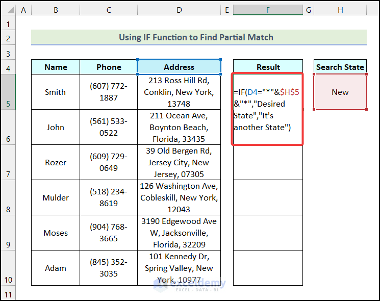
- Enter the formula in F5.
=IF(D4="*"&$H$5&"*","Desired State","It's another State")The asterisk sign (*) is used as a wildcard to denote that any number of characters can be returned. The value_if_true argument will return the partial match and the value_if_false argument will return “It’s another State”.
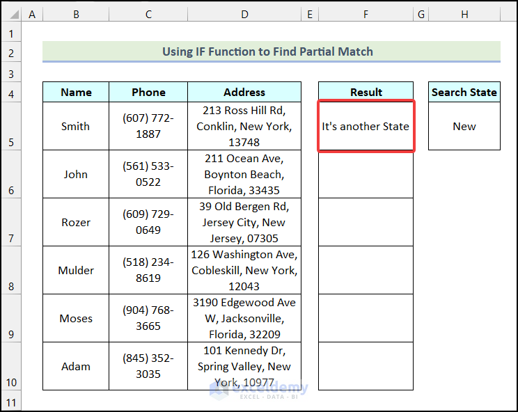
Although the cell contains “New”, the formula returned “It’s another State”. The IF function doesn’t work with wildcards.
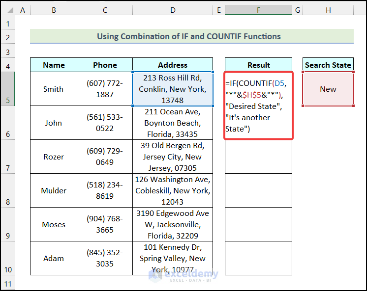
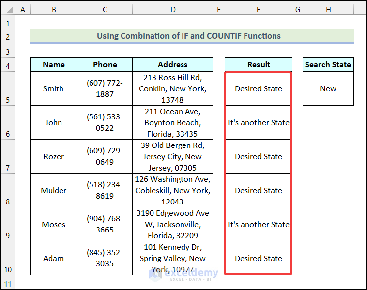
Method 1 – Combining the IF and the COUNTIF Functions to get a Partial Match in Excel
Steps:
- Enter the following formula in F5.
=IF(COUNTIF(D5,"*"&$H$5&"*"),"Desired State","It's another State")D5 is the selected Address, and H5 refers to the Search State.
Formula Breakdown
- In the COUNTIF(D5,”*”&$H$5&”*”) function,
- D5 → is the range argument.
- “*”&$H$5&”*” → is the criteria argument.
- Output → 1.
- In the IF function,
- COUNTIF(D5,”*”&$H$5&”*”) → is the logical_test argument.
- “Desired State” → is the [value_if_true] argument.
- “It’s another State” → is the [value_if_false] argument.
- Output → Desired State.
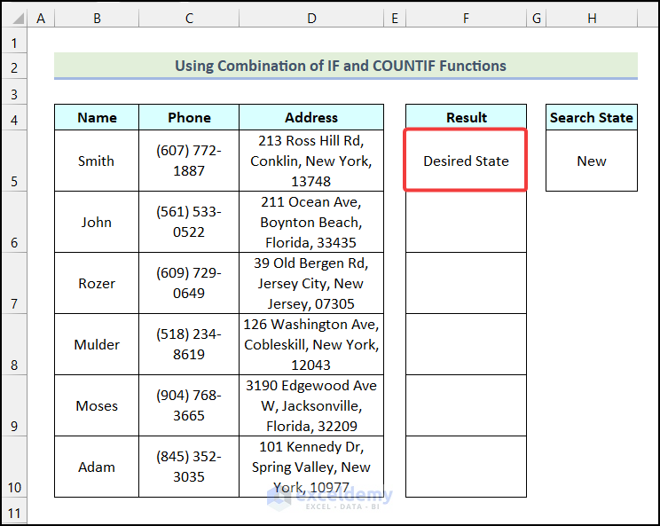
- Press ENTER.
You will see the following output in F5 as there is a partial match in D5.
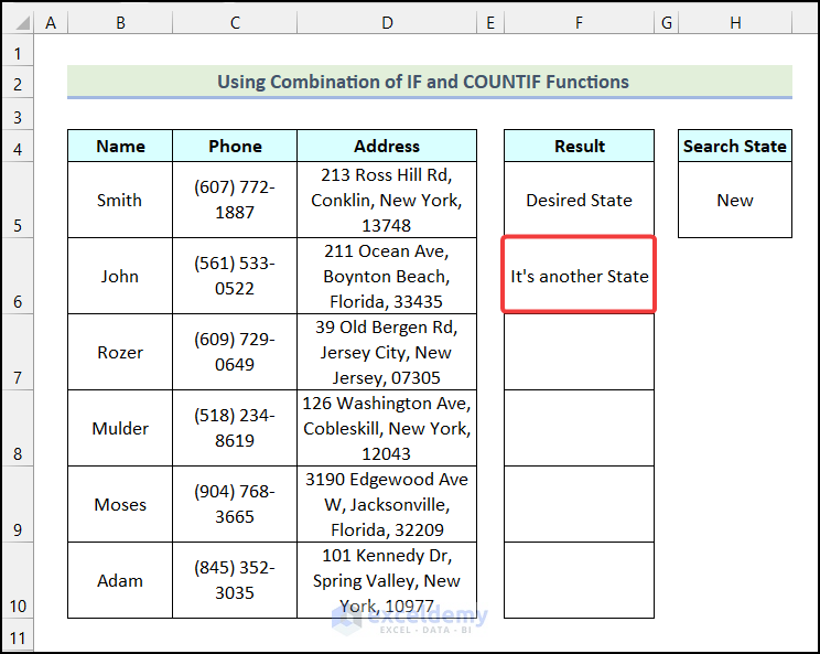
- Drag down the Fill Handle to the next cell to see the result.
The formula returned “It’s another state”, as there was no partial match.
- Drag down the Fill Handle to the next cell to see the result.
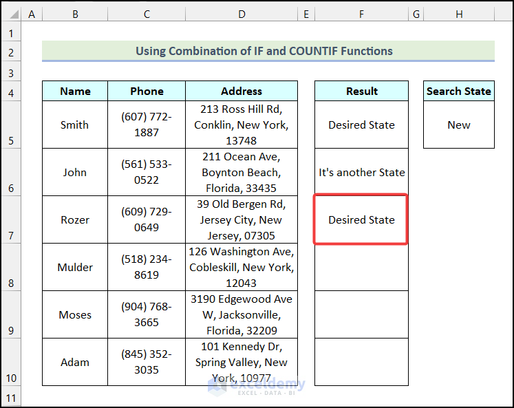
- Drag down the Fill Handle to see the result in the rest of the cells.
There are partial matches in F5, F7, F8, and F10.
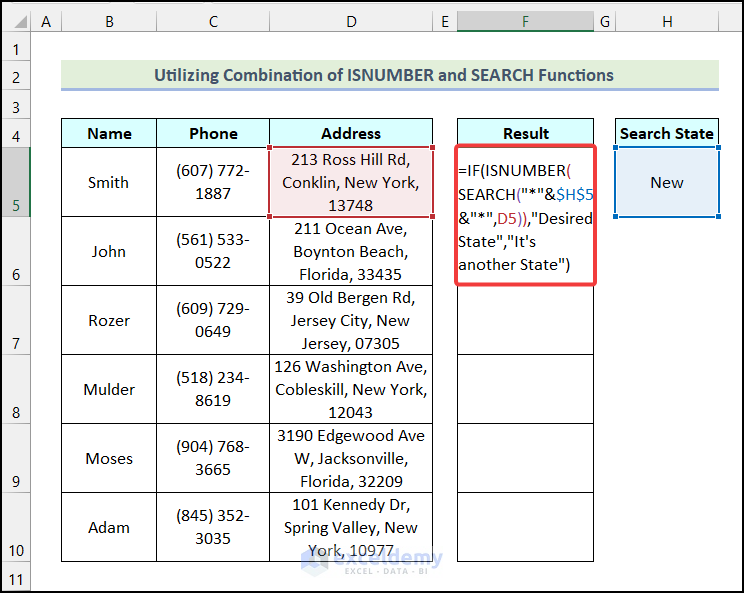
Method 2 – Combining the Excel ISNUMBER and SEARCH Functions to get a Partial Match
Steps:
- Enter the following formula in F5.
=IF(ISNUMBER(SEARCH("*"&$H$5&"*",D5)),"Desired State","It's another State")Formula Breakdown
- SEARCH(“*”&$H$5&”*”,D5) → returns the location of a text string inside another one.
- “*”&$H$5&”*” → is the find_text argument.
- D5 → is the within_text argument.
- Output → 1.
- ISNUMBER(SEARCH(“*”&$H$5&”*”,D5)) → becomes ISNUMBER(1).
- Output → TRUE.
- In the IF function,
- ISNUMBER(SEARCH(“*”&$H$5&”*”,D5)) → is the logical_test argument.
- “Desired State” → is the [value_if_true] argument.
- “It’s another State” → is the [value_if_false] argument.
- Output → Desired State.
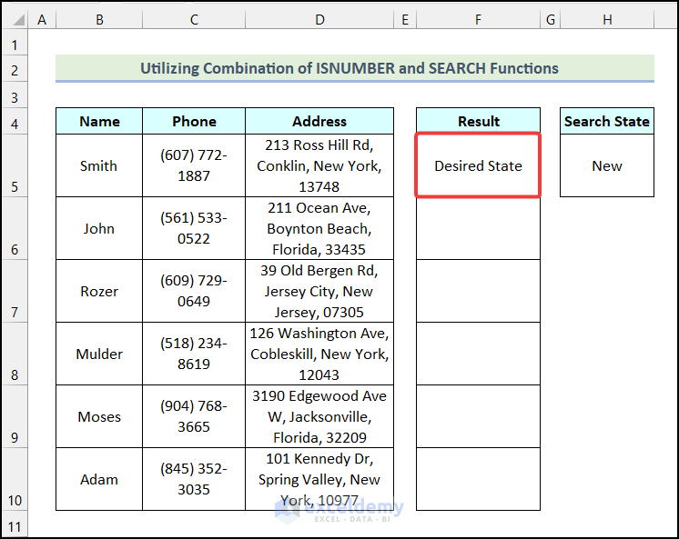
- Press ENTER.
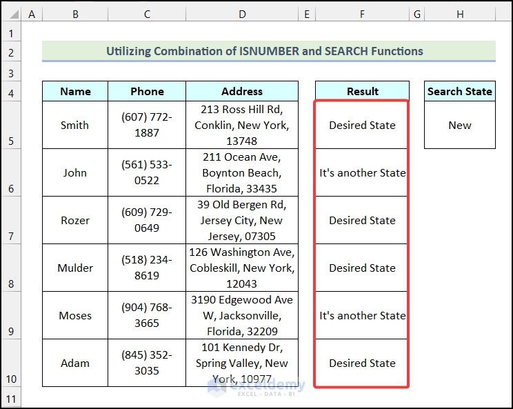
You will see the following output in F5:
- Drag down the Fill Handle to see the result in the rest of the cells.
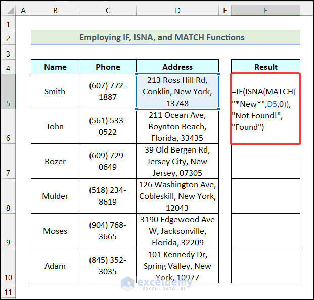
Method 3 – Merging the IF, ISNA, and MATCH Functions to get a Partial Match
Steps:
- Enter the following formula in F5.
=IF(ISNA(MATCH("*New*",D5,0)),"Not Found!","Found")Formula Breakdown
- MATCH(“*New*”,D5,0) → returns the relative position of a specified lookup value.
- Here, “*New*” → is the lookup_value argument.
- D5 → is the lookup_array argument.
- 0 → is the [match_type] argument.
- Output → 1.
- ISNA(MATCH(“*New*”,D5,0)) → becomes ISNA(1).
- Output → FALSE.
- In the IF function,
- ISNA(MATCH(“*New*”,D5,0)) → is the logical_test argument.
- “Not Found!” → is the [value_if_true] argument.
- “Found” →is the [value_if_false] argument.
- Output → Found.
- Press ENTER.
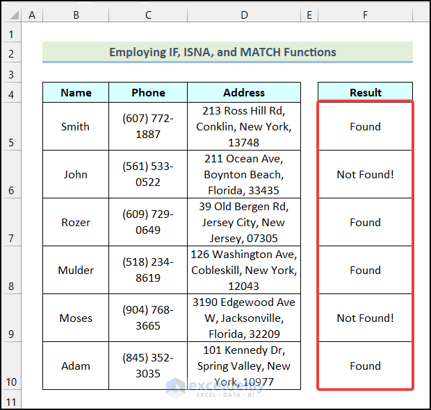
You will see the following output in F5:

- Drag down the Fill Handle to see the result in the rest of the cells.
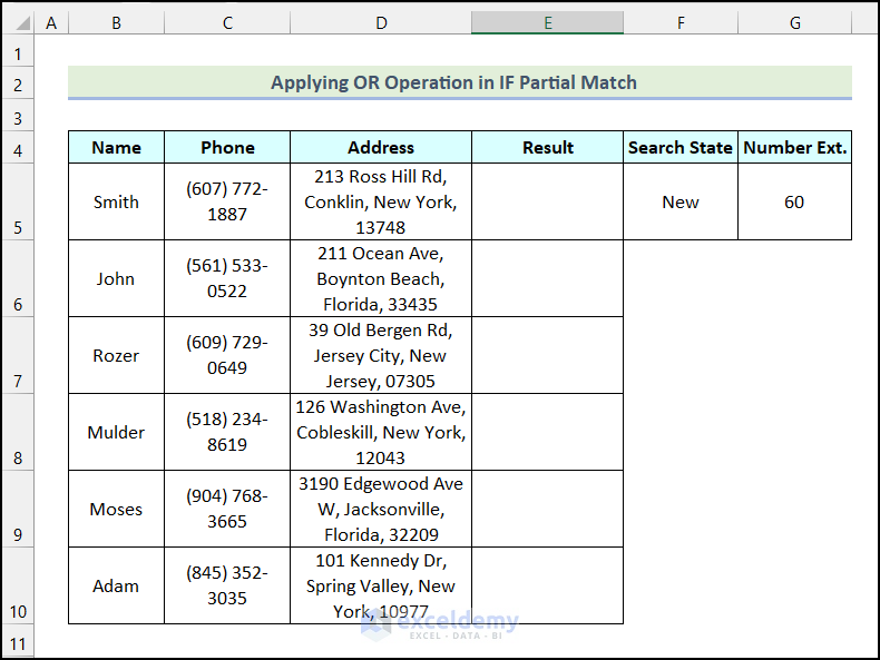
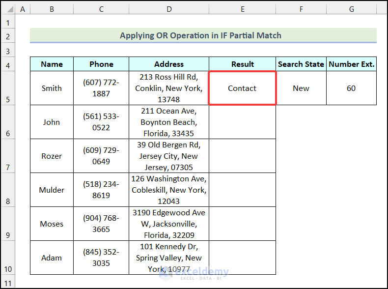
Method 4 – Applying the OR Operation with the IF Function to get a Partial Match
Steps:
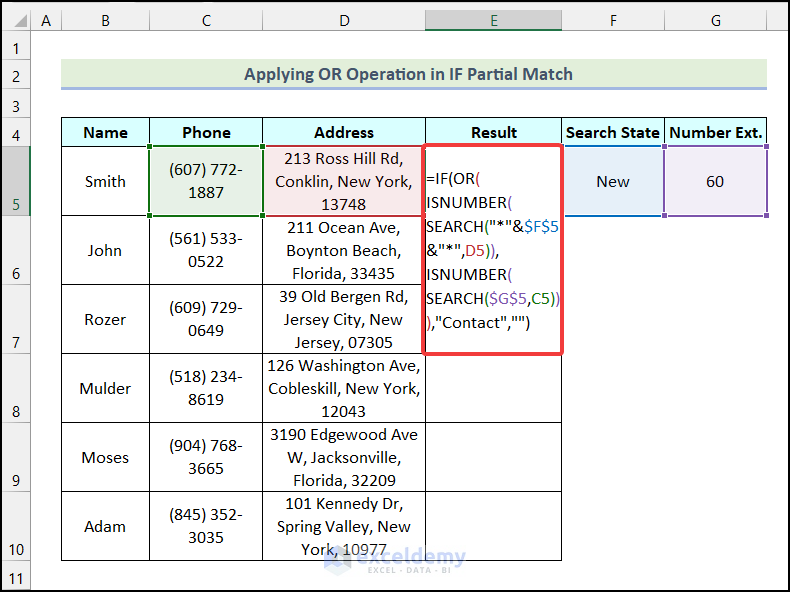
- Enter the following formula in E5.
=IF(OR(ISNUMBER(SEARCH("*"&$F$5&"*",D5)),ISNUMBER(SEARCH($G$5,C5))),"Contact","")F5 indicates the Search State, G5 refers to the Number Ext., and C5 is the first cell in the Phone column.
Formula Breakdown
- The two logical arguments of the OR function are:
- ISNUMBER(SEARCH(“*”&$F$5&”*”,D5)) → returns TRUE.
- ISNUMBER(SEARCH($G$5,C5)) → returns TRUE.
- OR(ISNUMBER(SEARCH(“*”&$F$5&”*”,D5)),ISNUMBER(SEARCH($G$5,C5))) → becomes OR(TRUE,TRUE).
- Output → TRUE.
- In the IF function,
- OR(ISNUMBER(SEARCH(“*”&$F$5&”*”,D5)),ISNUMBER(SEARCH($G$5,C5))) → is the logical_test argument.
- “Contact” → is the [value_if_true] argument.
- “” → is the [value_if_false] argument.
- Output → Contact.
- Press ENTER.
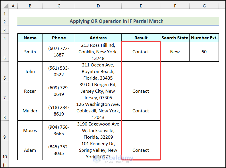
You will see the following output in E5:
- Drag down the Fill Handle to see the result in the rest of the cells.
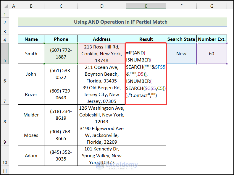
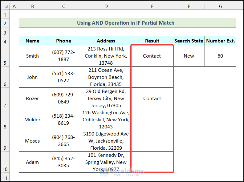
Method 5 – Using the AND Operation with an Excel IF Function to get a Partial Match
Steps:
- Enter the following formula in E5.
=IF(AND(ISNUMBER(SEARCH("*"&$F$5&"*",D5)),ISNUMBER(SEARCH($G$5,C5))),"Contact","")Formula Breakdown
- The two logical arguments of the AND function are:
- ISNUMBER(SEARCH(“*”&$F$5&”*”,D5)) → returns TRUE.
- ISNUMBER(SEARCH($G$5,C5)) → returns TRUE.
- AND(ISNUMBER(SEARCH(“*”&$F$5&”*”,D5)),ISNUMBER(SEARCH($G$5,C5))) → becomes AND(TRUE,TRUE).
- Output → TRUE.
- In the IF function,
- AND(ISNUMBER(SEARCH(“*”&$F$5&”*”,D5)),ISNUMBER(SEARCH($G$5,C5)) → is the logical_test argument.
- “Contact” → is the [value_if_true] argument.
- “” → is the [value_if_false] argument.
- Output → Contact.
- Press ENTER.
You will see the following output in E5, as both logical arguments return TRUE:
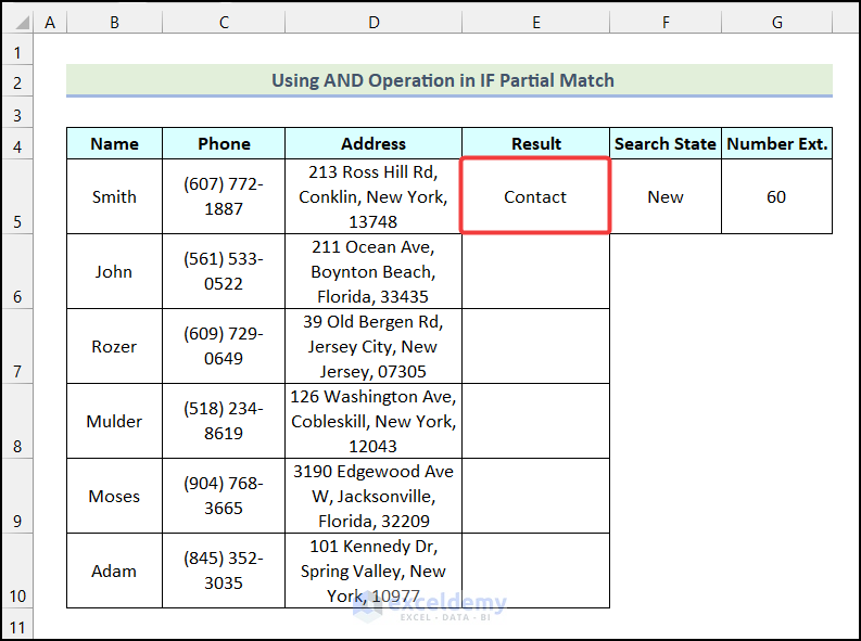
- Drag down the Fill Handle to see the result in the rest of the cells.
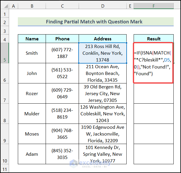
Method 6 – Finding a Partial Match using a Question Mark
Steps:
- Enter the following formula in F5.
=IF(ISNA(MATCH("*C?bleskill*",D5,0)),"Not Found!","Found")Formula Breakdown
- MATCH(“*C?bleskill*”,D5,0) → returns the relative position of a specified lookup value.
- “*C?bleskill*” → is the lookup_value argument.
- D5 → is the lookup_array argument.
- 0 → is the [match_type] argument.
- Output → #N/A.
- ISNA(MATCH(“*C?bleskill*”,D5,0)) → becomes ISNA(#N/A).
- Output → TRUE.
- In the IF function,
- ISNA(MATCH(“*C?bleskill*”,D5,0)) → is the logical_test argument.
- “Not Found!” → is the [value_if_true] argument.
- “Found” → is the [value_if_false] argument.
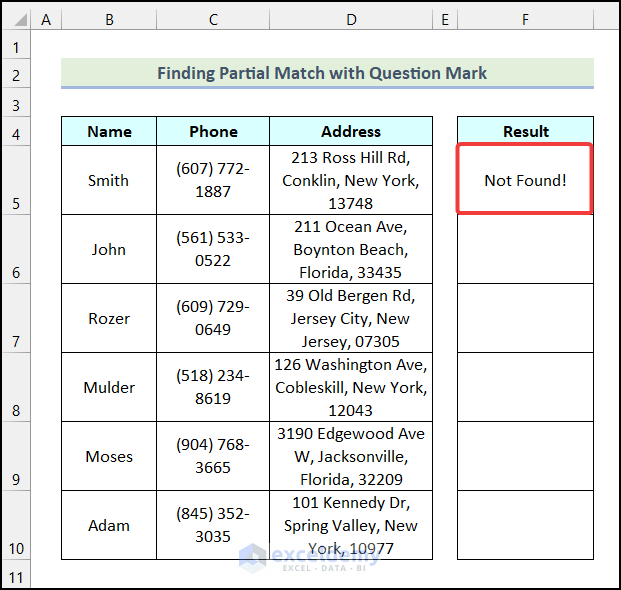
- Output → Not Found!.
- Press ENTER.
This is the output.
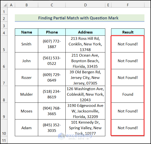
- Drag down the Fill Handle to see the result in the rest of the cells.
A partial match was found in D8 and the correct spelling is Cobleskill.
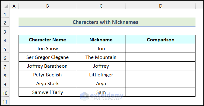
How to Find a Partial Match in Two Columns in Excel
The dataset contains Characters and Nicknames.
Steps:
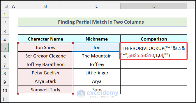
- Enter the following formula in D5.
=IFERROR(VLOOKUP("*"&C5&"*",$B$5:$B$10,1,0),"")C5 indicates the first cell in the Nickname column, and B5:B10 refers to the cells in the Character Name column.
Formula Breakdown
- The VLOOKUP function returns the value from the specified column if the value matches the lookup value.
- In the VLOOKUP(“*”&C5&”*”,$B$5:$B$10,1,0) function,
- “*”&C5&”*” → is the lookup_value argument.
- $B$5:$B$10 → is the table_array argument.
- 1 → is the col_index_num argument.
- 0 → is the [range_lookup] argument.
- Output → “Jon Snow”.
- The IFERROR function returns a specific value for the error criteria.
- IFERROR(VLOOKUP(“*”&C5&”*”,$B$5:$B$10,1,0),””) → becomes IFERROR(“Jon Snow”,””).
- “Jon Snow” → is the value argument.
- “” → is the value_if_error argument.
- Output → Jon Snow.
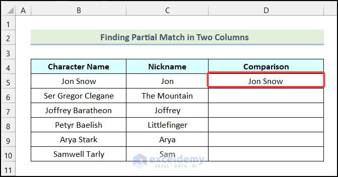
- Press ENTER.
This is the output.
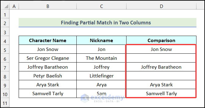
- Drag down the Fill Handle to see the result in the rest of the cells.
Download Practice Workbook
<< Go Back to Partial Match Excel | Formula List | Learn Excel
Get FREE Advanced Excel Exercises with Solutions!
