Download the Practice Workbook
8 Methods to Perform a Partial Match for a String in Excel
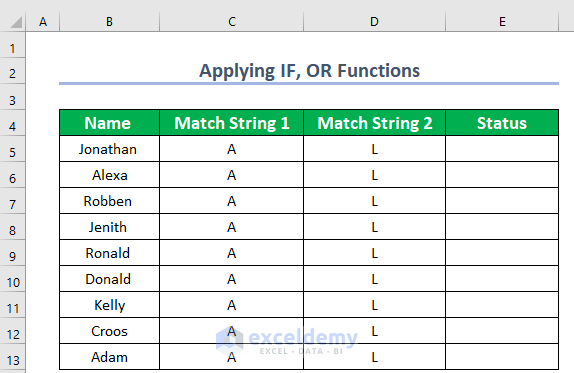
Method 1 – Using IF and OR Statement to Perform a Partial Match for String
The IF function does not support wildcard characters. Combining IF with other functions can be used for a partial match.
We have a data table where the names of some candidates are given in the Name column. We need to identify the names that contain one of the text strings given in columns 2 and 3.
Steps:
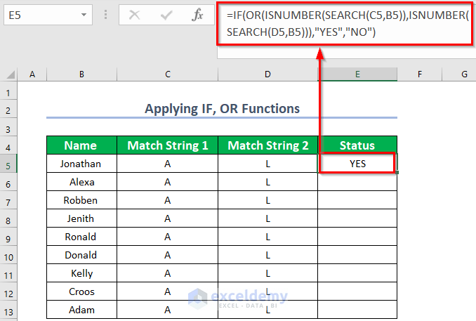
- In cell E5, apply the following formula:
- Insert the values into the formula:
=IF(OR(ISNUMBER(SEARCH(C5,B5)),ISNUMBER(SEARCH(D5,B5))),"YES","NO")
Formula Breakdown
- The text is C5 (A), D5 (L). The SEARCH will try to find the strings inside the cell.
- The cell is B5 (Jonathan).
- Value_if_true is “YES”.
- Value_if_false is “NO”.
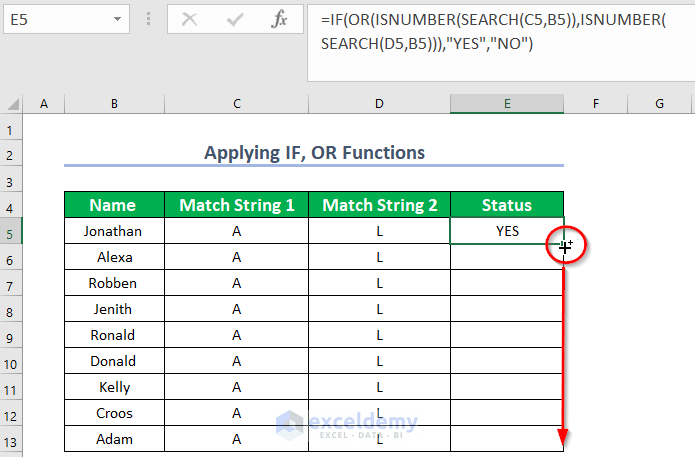
- Press Enter.
- Drag the Fill Handle icon down to AutoFill the corresponding formula into the rest of the cells.
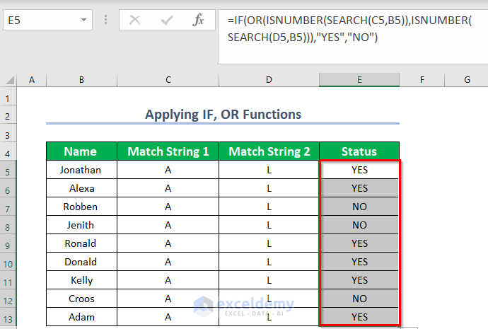
- Here’s the result.
Read More: How to Find Partial Match in Two Columns in Excel (4 Methods)
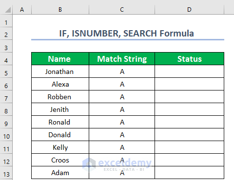
Method 2 – Use IF, ISNUMBER, and SEARCH Functions for a Partial Match
Consider a data set containing the columns Name, Match String, and Status. We need to identify the names that contain the string from the column Match String.
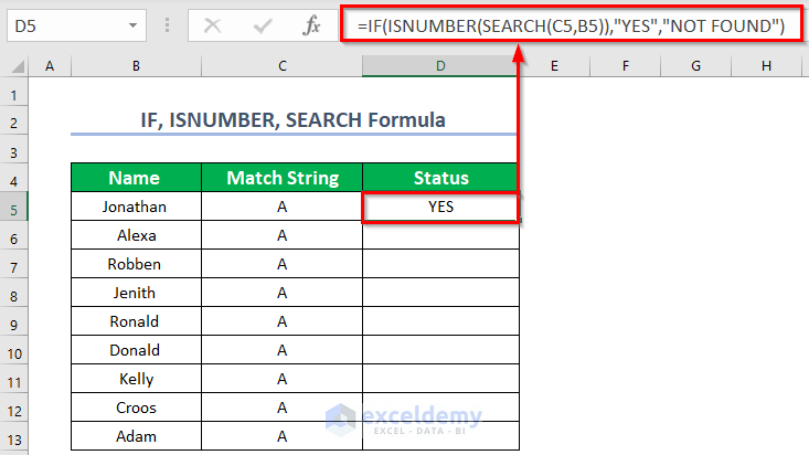
- Apply the formula with the IF, ISNUMBER, and SEARCH functions in the “Status” column in cell D5:
- After changing for the values in the sample, the formula is:
=IF(ISNUMBER(SEARCH(C5,B5)),"YES","NOT FOUND")- Press Enter.
Formula Breakdown
- The text is C5 (A). The formula will check whether C5 is inside the cell.
- The cell is B5 (Jonathan).
- Value_if_true is “YES”.
- Value_if_false is “NOT FOUND”.
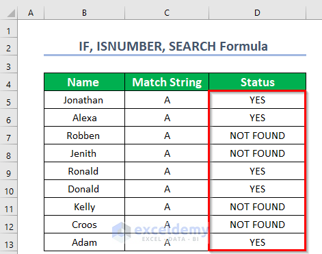
- Apply this formula for all the cells in the column to find out all the results that contain a partial match string.
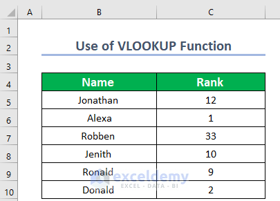
Method 3 – Using the VLOOKUP Function to Perform a Partial Match
Let’s consider a table where the names of some candidates and their ranks are given.
- Copy the column headers and paste them elsewhere in the worksheets.

- Insert the strings into the Name column in the new table. These will be the search values.
- Apply the VLOOKUP function in the F5 cell:
=VLOOKUP($E$5&"*",$B$5:$C$10,2,FALSE)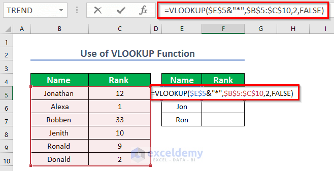
Formula Breakdown
- Lookup_value is $E$5&”*”. We used the Asterisk (*) as a wildcard that matches zero or more characters.
- Table_array is $B$5:$C$10.
- Col_index_num is 2.
- [range_lookup] is FALSE as we want the exact match.
- Press Enter.

- Drag the formula down to the other cells in the column.

Read More: How to Use VLOOKUP for Partial Match in Excel (4 Suitable Ways)
Similar Readings
- How to Use VLOOKUP to Find Approximate Match for Text in Excel
- Fuzzy Lookup in Excel (With Add-In & Power Query)
- Excel VLOOKUP to Find the Closest Match (with 5 Examples)
- How to Use Partial VLOOKUP in Excel (5 Suitable Examples)
- Excel SUMIF with Partial Match (3 Easy Ways)
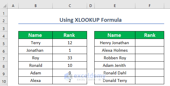
Method 4 – Incorporating the XLOOKUP Function to Perform a Partial Match
In the first table, the partial match strings are given with rank. We need to identify the names in the second table that contain the partial match strings and then return the rank associated with those names.
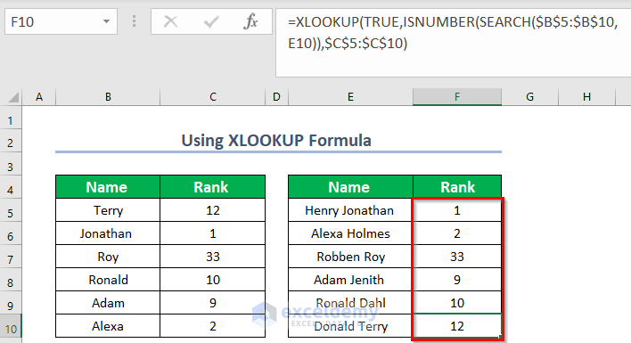
- In cell F5, apply the formula.
- After inserting the values, the formula becomes:
=XLOOKUP(TRUE,ISNUMBER(SEARCH($B$5:$B$10,E5)),$C$5:$C$10)- Hit Enter.

Formula Breakdown
- lookup_value is “TRUE”.
- The text is $B$5:$B$10.
- The cell is E5 (Henry Jonathan). The formula in the first cell will return the rank for Henry Jonathan.
- return_array is $C$5:$C$10.
- AutoFill to the other cells.
Read More: Lookup Partial Text Match in Excel (5 Methods)
Method 5 – Using the INDEX-MATCH Formula to Perform Partial Matching
In the first table, the Name and Rank of some candidates are given. In the second table, a partial match string is given. We need to identify the names from the first table that contains the partial match strings.
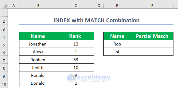
- In cell F5, apply the formula:
=INDEX($B$5:$B$10,MATCH(E5&"*",$B$5:$B$10,0))- Hit Enter.
We got the Name “Robben” which contains the partial match string (Rob).

Formula Breakdown
- The array is $B$5:$B$10.
- lookup_value is E5&”*”. We used the Asterisk (*) as a wildcard that matches zero or more characters.
- lookup_array is $B$5:$B$10.
- [match_type] is EXACT (0).
The Asterisk(*) can be used on both sides of the cell if you expect characters on both sides of your partial match string.
- Use the following formula in the F6 cell.
=INDEX($B$5:$B$10,MATCH("*"&E6&"*",$B$5:$B$10,0))- Press Enter to get the result.

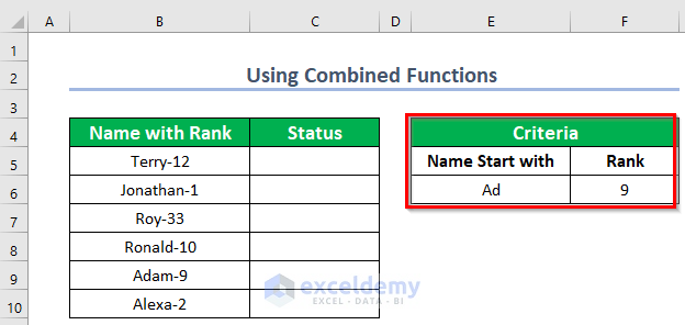
Method 6 – Combined Functions to Perform a Partial Match with Two Columns
We have two criteria that we need to match by.
Steps:
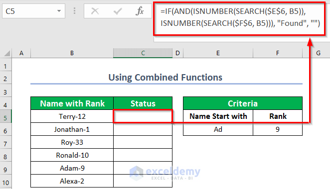
- Select a new cell C5 where you want to keep the status.
- Use the formula below in the C5 cell.
=IF(AND(ISNUMBER(SEARCH($E$6, B5)), ISNUMBER(SEARCH($F$6, B5))), "Found", "")- Hit Enter to get the result.
Formula Breakdown
- SEARCH($F$6, B5) will search if there are any strings Ad in the B5 cell.
- Output: #VALUE!.
- The ISNUMBER function will check whether the above output is a number or not.
- Output: FALSE.
- ISNUMBER(SEARCH($E$6, B5)) will do the same for the second partial match string.
- Output: FALSE.
- The AND function will check whether both values are TRUE.
- Output: FALSE.
- The IF function will return “Found” if AND returns TRUE. Otherwise, it will return a void cell.
- Output: The output is blank/empty as there is no match for the string value of the B5 cell.
- Drag the Fill Handle icon to AutoFill the formula in the rest of the cells.

Read More: How to Use IF Function to Find Partial Match in Excel (6 Ways)
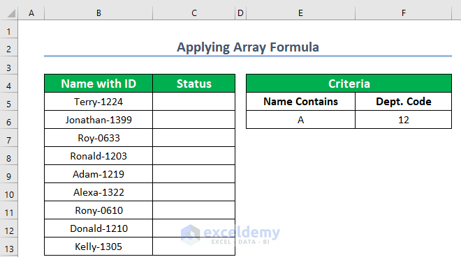
Method 7 – Applying an Array Formula to Find a Partial Match with Two Columns
We have two criteria to use for partial matches.
Steps:
- Select cell C5.
- Insert the following formula:
=IF(COUNT(SEARCH({"A","12"}, B5))=2, "Found", "")- Press Enter to get the result.

Formula Breakdown
- SEARCH({“A”,”12″}, B5) will search for the string A and the number 12 in the B5 cell.
- Output: {#VALUE!,7}.
- The COUNT function will count the number of “hits” in the cell.
- Output: 1.
- The IF function will return “Found” if the COUNT function returns 2. Otherwise, it will return a void cell.
- Output: The output is blank/empty as there is only one match, but we need two.
- Drag the Fill Handle icon to AutoFill the corresponding data in the rest of the cells.

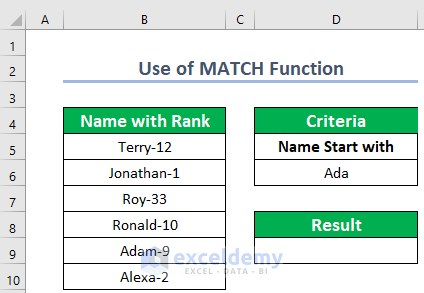
How to Get the Position of a Partial Match in Excel
We have to extract the partial string from the “Name with Rank” column and locate where it is in the searched list.
Steps:
- Use the formula given below in the D9 cell.
=MATCH("*"&D6&"*", B5:B10, 0)- Press Enter to get the result.

Formula Breakdown
- lookup_value is “*”&D6&”*”.
- lookup_array is B5:B10.
- [match_type] is EXACT (0).
Read More: How to Use INDEX and Match for Partial Match (2 Easy Ways)
Things to Remember
✅ The XLOOKUP function is only available in Microsoft 365 version. So, only the users of Excel 365 can use this function.
✅ The VLOOKUP function always searches for lookup values from the leftmost top column to the right. Moreover, this function never fetches data on the left.
✅ The Asterisk(*) is used as a wildcard. Use it on both sides of the partial match string if you need wildcard characters on both sides.
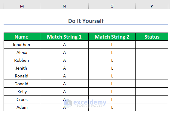
Practice Section
We’ve included a practice section you can use to test these methods.
Further Readings
- How to Use COUNTIF Function for Partial Match in Excel
- Conditional Formatting for Partial Text Match in Excel (9 Examples)
- How to Use VLOOKUP to Find Partial Text from a Single Cell
- Highlight Partial Text in Excel Cell (9 Methods)

