This is the syntax of the VLOOKUP function:
VLOOKUP (lookup_value, table_array, column_index_num, [range_lookup])
The fourth argument (range_lookup) indicates whether we are looking for the exact match or an approximate match:
- FALSE: To get an exact match.
- TRUE: To get an approximate match.
If the lookup column contains text values, the function will not return an approximate match. You need to use a wildcard in the first argument. Here, the asterisk (*).
Example 1 – Applying a Wildcard in VLOOKUP to Find a Partial Match (Text Begins with)
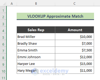
The dataset showcases sales representatives’ names and their sales amounts. To search for the sales representative’s name beginning with ‘Brad’ and see the corresponding sales amount:
Steps:
- Enter the formula in C14.
=VLOOKUP(C12&"*",B5:C10,2,FALSE)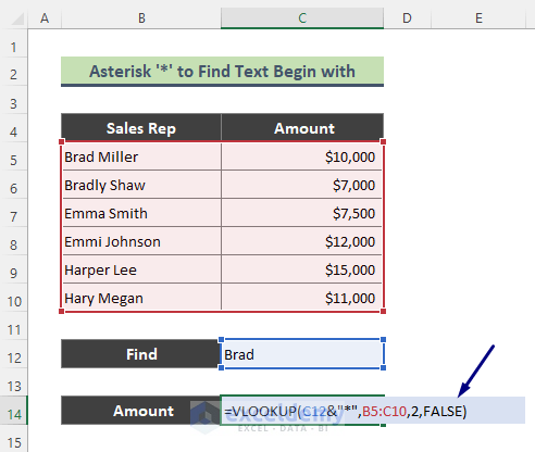
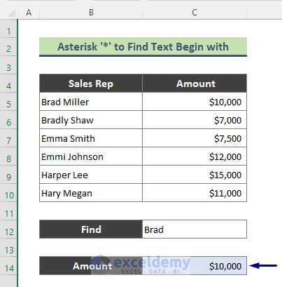
- Press Enter.
This is the output.
Formula Breakdown
C12&”*”
The Ampersand (&) joins the value of C12 (Brad) with the wildcard (*). The lookup value becomes Brad*. The VLOOKUP formula looks for the text that begins with Brad*: names starting with Brad, with zero or more characters (eg. Brad, Bradley, Braden).
VLOOKUP(C12&”*”,B5:C10,2,FALSE)
The formula looks for Brad* in B5:C10 and returns the sales amount in column 2. FALSE in the fourth argument indicates that the exact match mode is used.
Note:
Be careful with duplicates. The dataset contains two names beginning with Brad: Brad Miller and Bradly Shaw. If multiple partial matches are found, the formula will return the first match only.
Read More: Use VLOOKUP to Find Partial Text from a Single Cell
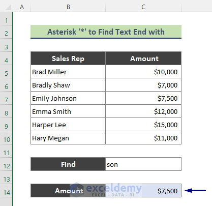
Example 2 – Finding an Approximate Match when the Cell Value Ends with a specific Text
To search sales representative’s names that end with ‘son’ and see their sales amount:
Steps:
- Enter the formula in C14.
=VLOOKUP("*"&C12,B5:C10,2,FALSE)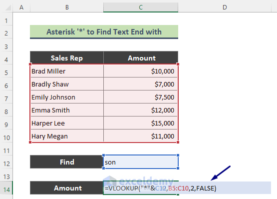
- It looks for the sales representative name ending with ‘son’ and returns the corresponding sales amount ($7,500) after pressing Enter.
“*”&C12, returns *son. The rest of the formula works as mentioned in Example 1.
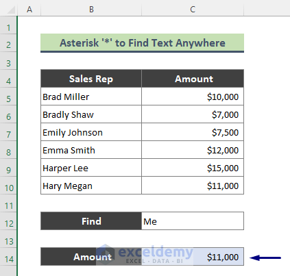
Example 3 – Using Two Wildcards in the VLOOKUP Function to Get a ‘Contains Type’ Partial Match
To search for the sales representative’s names containing ‘Me’ at any position and find the sales amount:
Steps:
- Enter the formula in C14.
=VLOOKUP("*"&C12&"*",B5:C10,2,FALSE)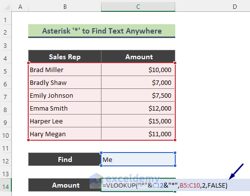
- The formula will look for the sales representative’s names containing ‘Me’ and return the sales amount ($11,000) after pressing Enter.
“*”&C12&”*”, returns *Me*.
Read More: How to Perform VLOOKUP with Wildcard in Excel
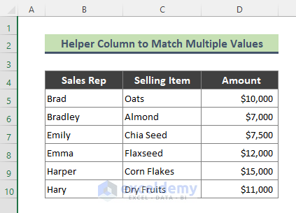
Example 4 – Getting an Approximate Match in Multiple Texts with a Helper Column and the VLOOKUP Function
The dataset showcases Sales Rep, Selling Item, and Sales Amount.
Steps:
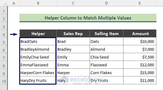
- Create a ‘helper column’ to concatenate the values of columns C and D by entering the formula in B5.
=C5&D5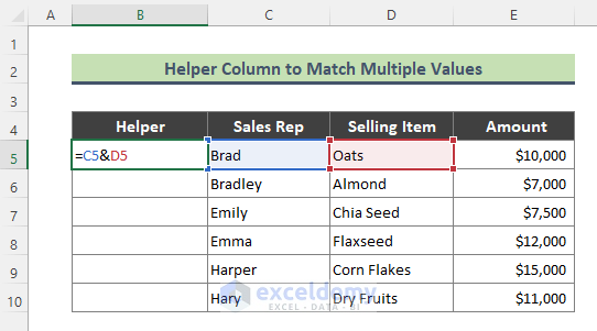
- Drag down the Fill Handle to see the result in the rest of the cells.
To look for the value of C12 and C13 in the helper column:
- Enter the following formula in C15.
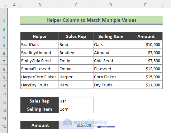
=VLOOKUP(C12&"*"&C13&"*",$B$5:$E$10,4,0)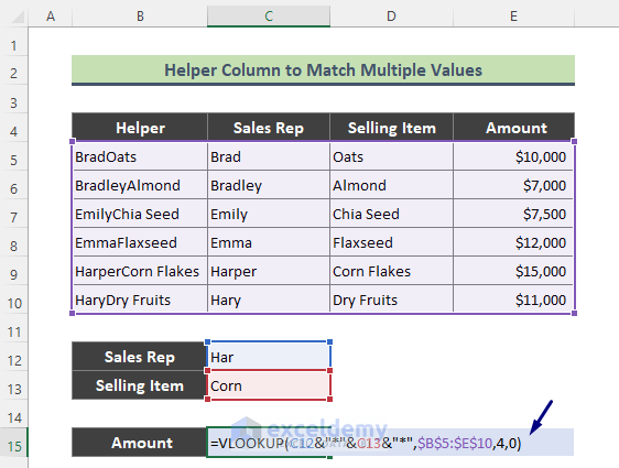
- Press Enter.
This is the output.
Read More: Use VLOOKUP to Find Multiple Values with Partial Match in Excel
Alternatives to the Vlookup Function to Get an Approximate Match for a Text
Microsoft has a free add-in: Fuzzy Lookup.
Download Practice Workbook
Download the practice workbook.
Related Articles
- How to Vlookup Partial Match for First 5 Characters in Excel
- How to Use Excel VLOOKUP to Find the Closest Match
- Excel VLOOKUP for Partial Match in Table Array
<< Go Back to VLOOKUP Partial Match | Excel VLOOKUP Function | Excel Functions | Learn Excel
Get FREE Advanced Excel Exercises with Solutions!
