Circumstances may demand a partial match with multiple values. Our agenda for today is to assist you in performing a partial match using VLOOKUP with multiple values. This article will demonstrate how to determine multiple values with a partial match using VLOOKUP in Excel. First things first, let’s get to know about the workbook, which is the basis of our examples.
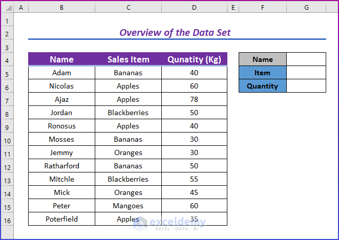
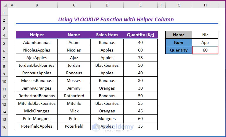
Here, we have a table of several salespeople along with their sales items and quantities. Using this data, we will perform a partial match with multiple values.

How to Use VLOOKUP Function in Excel for Extracting Multiple Values with Partial Match: 2 Handy Approaches
Here in our examples, to keep things straightforward, we will use two values while finding the matches. Besides, we will provide the name and item value, and in return, we will get the quantity. Since our formula will be based on the VLOOKUP function, you can check the function in this article; “The VLOOKUP function”. Firstly, we will use a helper column and the CHOOSE function, incorporating the VLOOKUP function, to find the multiple values from a partial match. Additionally, we will apply multiple functions, such as INDEX, MATCH, AGGREGATE, and ROW functions, to achieve the same task.
Method 1: Using VLOOKUP Function with Helper Column for Finding Multiple Values with Partial Match in Excel
In this section, we will show how to perform a partial match with multiple values using a helper column with the VLOOKUP function by providing the name and item value, and in return, we will get the quantity.
Steps:
- Firstly, select the B5 cell.
- After that, write down the following formula below.
=C5&D5- Then, press Enter.
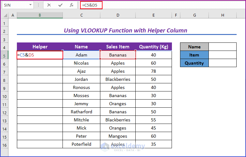
- Therefore, the helper column will be filled by concatenating the original column of the lookup values. The concatenation can be done using the ampersand (&) sign.
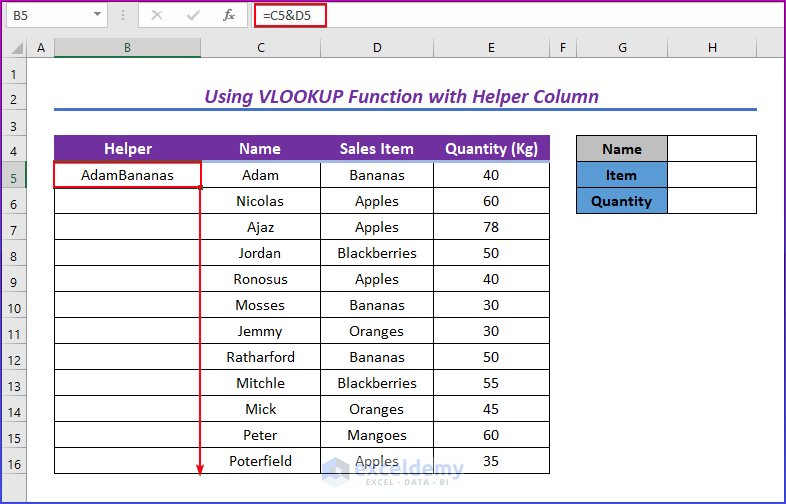
- After that, filling up the helper column let’s add the two criteria values.
- So, the provided values are Adam and Banana. You can see the initial table doesn’t have the item Banana, so we need to build the formula in such a way that it will return value in this kind of case.
- Lastly, we will apply the below formula in the H6 cell.
=VLOOKUP(H4&"*"&H5&"*",$B$5:$E$16,4,0)- Here, H4 and H5 are the values to look at.
- Then, press Enter.
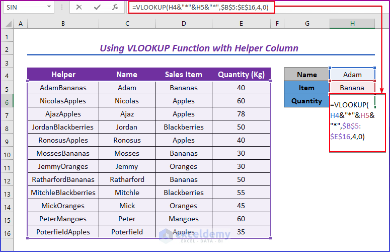
- And the asterisk (*) sign is the wildcard. When there is an asterisk sign, it denotes that any number of characters (including 0) can take the place.
- Here we have used two asterisks, one within the two values and another one at the end of the values. Hope you have understood that we have concatenated these together before starting to search within the lookup_array.
- Our desired result is within the 4th column, so we used 4 in the column_num.
- It provided the number of bananas sold (Though we had set Bananas).

- Let’s change the values and see the updated result.
- Here we have set Nic and App at the Name and Item You can see no values listed in the original table.
- But it gave the values from Nicolas who sells As the provided values partially matched these values.
Read More: How to Use VLOOKUP to Find Partial Text from a Single Cell
Method 2: Combining CHOOSE Function with VLOOKUP Function to Find Multiple Values with Partial Match
In this section, we will show how to perform the task without any helper column. This time we will use a helper function called the CHOOSE function. The CHOOSE function returns a value from a list using a given position or index.
The Syntax of the CHOOSE Function
=CHOOSE(index_num, value1, [value2], ...)The Argument of the CHOOSE Function
| Argument | Explanation |
|---|---|
| index_num | A number between 1 to 254, specifies the value argument. |
| value1 | A value from which to choose. |
| value2 | This is an optional field. |
- Firstly, choose the G6 cell.
- So, let’s write the formula to pass two lookup values.
=VLOOKUP(G4&"*"&G5&"*",CHOOSE({1,2},$B$5:$B$16&$C$5:$C$16,$D$5:$D16),2,0)- After that, press Enter.
- Here, the use of the two values and the wildcard is similar to the formula of the earlier section.
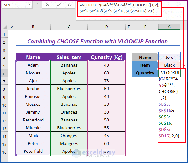
- The CHOOSE portion of this formula works as a virtual helper table. We have used 1 and 2 (within the curly braces) as the index number.
- Then, we concatenated the Name and Sales Item columns together, this will be the first column of our virtual table.
- Here, we have inserted the Quantity column in the value2 field, which will be the virtual table’s second column.
- This table becomes the lookup_array for the VLOOKUP function. Since our desired result would be found in the second column from the virtual table we have used 2 as the column_number.
- Here, our provided values are Jord and Black, and the formula derived values from Jordan and Blackberries.
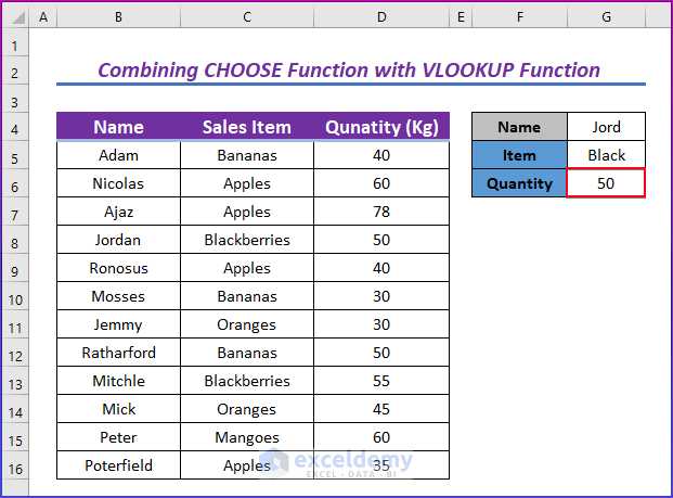
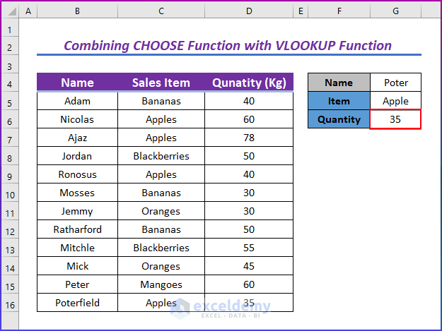
- Then, we will change the values to see the updated result.
- As a result, the values we have set are Poter and Apple (no such values in the list), the formula provided the value for Porterfield where it found the partial match.
Read More: Excel VLOOKUP for Partial Match in Table Array
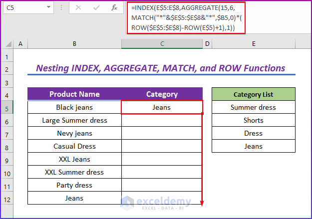
Nesting INDEX, AGGREGATE, MATCH, and ROW Functions for Extracting Multiple Values with Partial Match
Additionally, we can extract multiple data with partial matches without the assistance of the VLOOKUP function. To do this, we can define the values by performing a partial match operation. In this section, we will see how to match the category by performing a partial match. Here, we have some products and categories listed separately. We aim to compare the product name with the category name and name the category when it finds a match. You can see that hardly a product name can be exactly the same as the category, so a partial match is key.
This time we will use the INDEX – AGGREGATE combination. The INDEX function returns the value at a given location in an array or range. For further information, visit this article; INDEX. The AGGREGATE function returns an aggregate calculation like AVERAGE, COUNT, MAX, etc.
The Syntax of the AGGREGATE Function
=AGGREGATE(function_number,behavior_options, range)The Argument of the AGGREGATE Function
| Argument | Explanation |
|---|---|
| function_number | This number specifies which calculation should be made |
| function_number | Set this by using a number. This number denotes how the function will behave. |
| range | The range you want to aggregate. |
The AGGREGATE function does several tasks, so a number of functions are predefined within it. We are listing a few frequently used function numbers
| Function | Function_number |
|---|---|
| AVERAGE | 1 |
| COUNT | 2 |
| COUNTA | 3 |
| MAX | 4 |
| MIN | 5 |
| PRODUCT | 6 |
| SUM | 9 |
| LARGE | 14 |
| SMALL | 15 |
Steps:
- Firstly, choose the C5 cell.
- Secondly, write down the following formula.
=INDEX(E$5:E$8,AGGREGATE(15,6,MATCH("*"&$E$5:$E$8&"*",$B5,0)*(ROW($E$5:$E$8)-ROW(E$5)+1),1))- Then, hit Enter.

- Firstly, the MATCH portion will match the rows with the product name and as we have declared 0 as the third argument, it will be considered an exact match.
- Afterward, E5:E8 is the array within which we need to find. Within AGGREGATE we have set 15 as function_number and 6 as behavior_option which stands for ignoring error values.
- Besides, the ROW functions provide the row number iteratively.
- Lastly, the INDEX function will figure out the data of the matched cell.
- Therefore, the formula provided the category name perfectly after comparing the product name and category list.
- Lastly, use the Fill Handle tool and drag it down from the C5 cell to the C12 cell.
- Finally, you will get the results in the below image.

Read more: How to Vlookup Partial Match for First 5 Characters in Excel
Download Practice Workbook
You may download the following Excel workbook for better understanding and practice it by yourself.
Conclusion
That’s all for today. We have tried listing several ways to perform the partial match using VLOOKUP with multiple values. Hope you will find this helpful. So, feel free to comment if anything seems difficult to understand. Let us know any other methods which we might have missed here.
Further Readings
- How to Use Excel VLOOKUP to Find the Closest Match
- How to Use VLOOKUP to Find Approximate Match for Text in Excel
- How to Perform VLOOKUP with Wildcard in Excel
- [Fixed!] Excel VLOOKUP Partial Match Not Working
<< Go Back to VLOOKUP Partial Match | Excel VLOOKUP Function | Excel Functions | Learn Excel
Get FREE Advanced Excel Exercises with Solutions!

Hi Shakil,
I like your answer using Index-Aggregate, but what does the formula look like if you want to look up the category and return whatever is in column F for that category?
Thanks.
Geoff
As far as I’ve understood you are wanting to get value with category criteria, where for different categories items under those categories will show up. I’ve tried to visualize that like the following.
you can get the Products with respect to the category by using the following formula
=IF(ROWS($F$5:F5)>$C$15,” “,INDEX($B$5:$B$12,AGGREGATE(15,6,(ROW($C$5:$C$12)-ROW($C$5)+1)/($C$5:$C$12=$E$5),ROWS($F$5:F5))))
The Count column is obtained using the COUNTIFS function. =COUNTIFS($C$5:$C$12,B15). Feel free to access the reply-workbook.