Overview of INDEX Function
- Description:
It returns a value or reference of the cell at the intersection of a particular row and column, in a given range.
- Generic Syntax:
INDEX (array, row_num, [column_num])
- Argument Description:
| ARGUMENT | REQUIREMENT | VALUE |
|---|---|---|
| array | Required | Pass a range of cells, or an array constant to this argument |
| row_num | Required | Pass the row number in the cell range or the array constant |
| col_num | Optional | Pass the column number in the cell range or the array constant |
Note:
- If you use both the row_num and column_num arguments, the INDEX function will return the value from the cell at the intersection of the row_num and column_num.
- If you set row_num or column_num to 0 (zero), you will get the whole column values or the whole row values respectively in the form of arrays. You can insert those values into cells using Array Formula.
Overview of AGGREGATE Function
- Description:
The AGGREGATE function is used on different functions like AVERAGE, COUNT, MAX, MIN, SUM, PRODUCT, etc., with the option to ignore hidden rows and error values to get certain results.
- Generic Syntax:
- Syntax with References:
AGGREGATE(function_num, options, ref1, ref2, …)
-
- Syntax with Array Formula:
AGGREGATE(function_num, options, array, [k])
- Arguments Description:
Arguments in the Reference form,
function_num = Required, operations to perform. There are 19 functions available to perform with the AGGREGATE function. Individual numbers define each function. (see the table below)
| Function Name | Function Number |
|---|---|
| AVERAGE | 1 |
| COUNT | 2 |
| COUNTA | 3 |
| MAX | 4 |
| MIN | 5 |
| PRODUCT | 6 |
| STDEV.S | 7 |
| STDEV.P | 8 |
| SUM | 9 |
| VAR.S | 10 |
| VAR.P | 11 |
| MEDIAN | 12 |
| MODE.SNGL | 13 |
| LARGE | 14 |
| SMALL | 15 |
| PERCENTILE.INC | 16 |
| QUARTILE.INC | 17 |
| PERCENTILE.EXC | 18 |
| QUARTILE.EXC | 19 |
options = Required, values to ignore. There are 7 values each representing the option to ignore while performing the operations with the functions defined.
| Option Number | Option Name |
|---|---|
| 0 or omitted | omit nested AGGREGATE and SUBTOTAL functions |
| 1 | omit hidden rows, nested SUBTOTAL, and AGGREGATE functions |
| 2 | leave out error values, nested SUBTOTAL, and AGGREGATE functions |
| 3 | omit hidden rows, error values, nested SUBTOTAL, and AGGREGATE functions |
| 4 | leave out nothing |
| 5 | leave out hidden rows |
| 6 | omit error values |
| 7 | Ignore hidden rows and error values |
ref1 = Required, the first numeric argument for functions to perform the operation. It could be one single value, array value, cell reference, etc.
ref2 = Optional, it could be numeric values from 2 to 253
Arguments in the Array Formula,
function_num = (as discussed above)
options = (as discussed above)
array = Required, range of numbers or cell references based on what the functions will perform.
[k] = Optional, this argument is needed only when performing with the function number from 14 to 19 (see the function_num table).
- Return Value
Return values based on the function specified.
How to Combine INDEX and AGGREGATE Functions in Excel
Example 1 – Using INDEX and AGGREGATE Functions for Calculating Sum in Excel
Steps:
- Arrange a dataset like the following image.
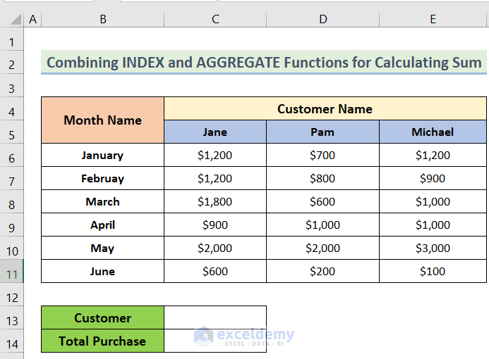
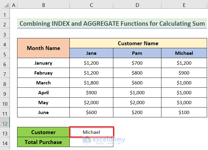
- In cell C13, insert the name of the desired customer.
- In cell C14, enter the following formula.
=AGGREGATE(9,0,INDEX(C6:E11,,MATCH(C13,C5:E5,0)))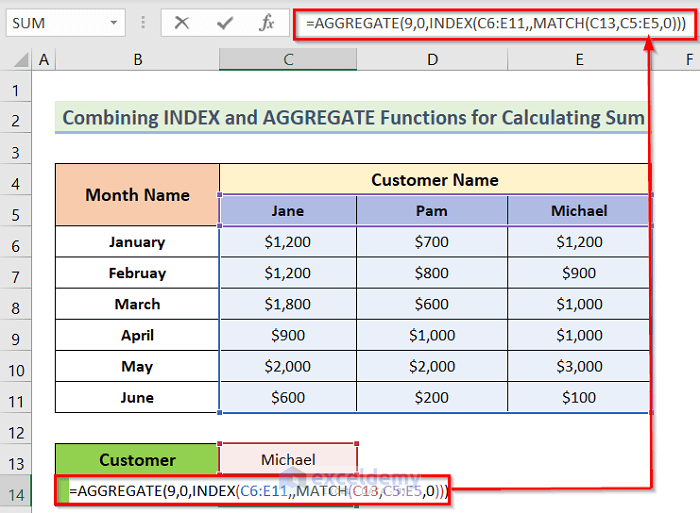
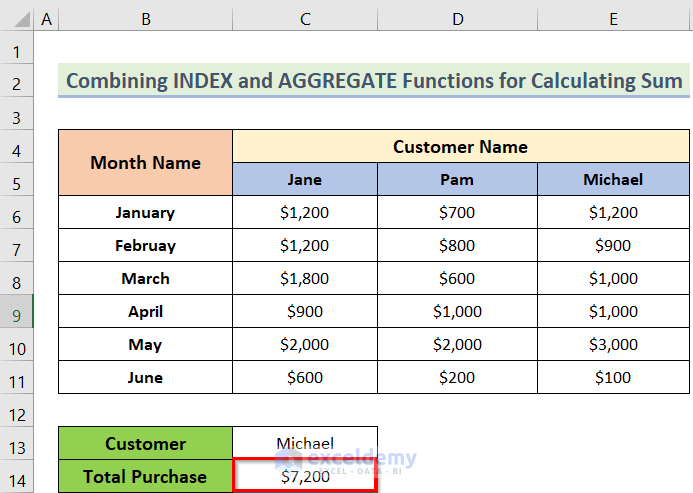
- You will get the desired result.
How Does the Formula Work?
- MATCH(C13, C5:E5,0): This represents the selected range of the cell you want to find a match from.
- INDEX(C6:E11, MATCH(C13, C5:E5,0)): This portion represents the count function the formula will work on.
- AGGREGATE(9,0,INDEX(C6:E11,,MATCH(C13,C5:E5,0)))): This represents the whole condition.
Read More: How to Aggregate Data in Excel
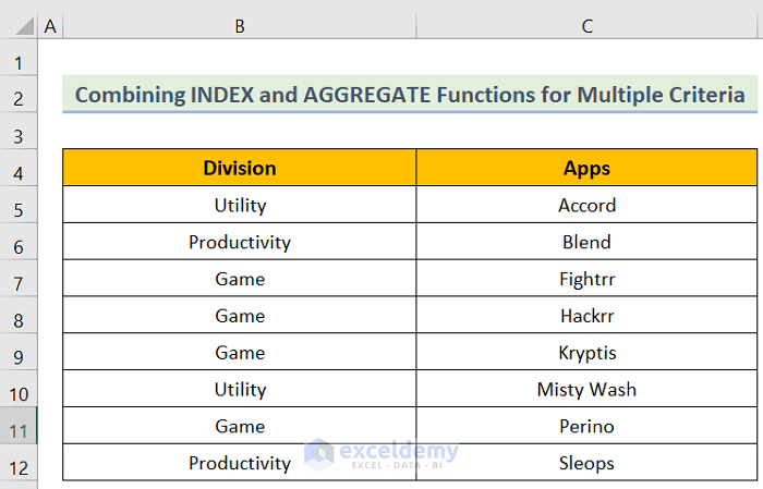
Example 2 – Combine INDEX and AGGREGATE Functions for Multiple Criteria
Steps:
- Arrange a dataset like the following image.
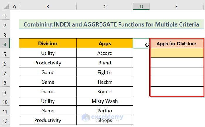
- Add one extra column in column E to show the output values.
- In cell D4, enter the following formula.
=COUNTIF($B$5:$B$12,$E$5)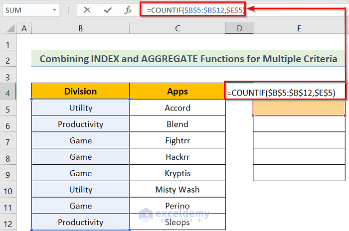
- Enter the desired division’s name in cell E5 and it will show the number of results in cell D4.
- In cell E6, insert the following formula.
=@IF(ROWS($D$5:D5)<=$D$4,INDEX($C$5:$C$12,AGGREGATE(15,3,($B$5:$B$12=$E$5)/($B$5:$B$12=$E$5)*(ROW($B$5:$B$12)-ROW($B$4)),ROWS($D$5:D5))),"")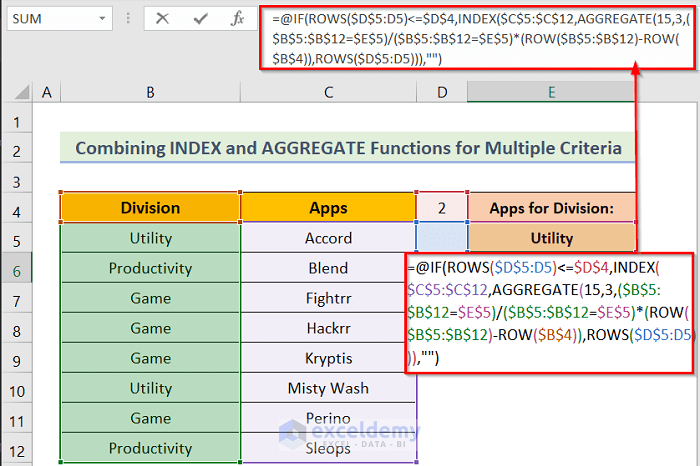
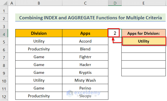
- Press the Enter button to get the result for the cell. Use the Fill Handle to apply the formula to all the desired cells.
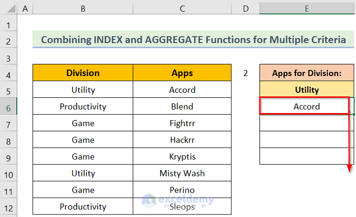
- You will get the desired result similar to the following image.
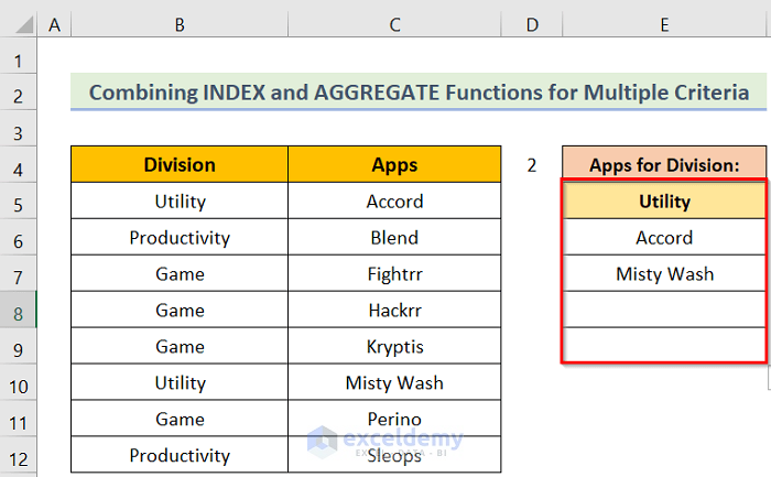
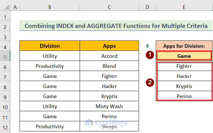
- When you make changes in cell C5, the result will update accordingly.
How Does the Formula Work?
- ROWS($D$5:D5): This represents the reference cell.
- AGGREGATE(15,3,($B$5:$B$12=$E$5)/($B$5:$B$12=$E$5)*(ROW($B$5:$B$12)-ROW($B$4)), ROWS($D$5:D5)): This represents the selected range of the database you want to use or find a match from.
- INDEX($C$5:$C$12, AGGREGATE(15,3,($B$5:$B$12=$E$5)/($B$5:$B$12=$E$5)*(ROW($B$5:$B$12)-ROW($B$4)), ROWS($D$5:D5))): This represents the function the formula will work on.
- IF(ROWS($D$5:D5)<=$D$4,INDEX($C$5:$C$12,AGGREGATE(15,3,($B$5:$B$12=$E$5)/($B$5:$B$12=$E$5)*(ROW($B$5:$B$12)-ROW($B$4)),ROWS($D$5:D5))),””): The total portion represents the whole condition.
Read More: How to Use Excel AGGREGATE Function with Multiple Criteria
Download Practice Workbook
Related Articles
- AGGREGATE Formula for Adding Serial Number in Excel
- How to Aggregate COUNTIF in Excel
- How to Use Conditional AGGREGATE Function in Excel
- Combining AGGREGATE with IF Function in Excel
- AGGREGATE vs SUBTOTAL in Excel
<< Go Back to Excel AGGREGATE Function | Excel Functions | Learn Excel
Get FREE Advanced Excel Exercises with Solutions!
