Microsoft Excel functions like SUM, COUNT, LARGE, and MAX won’t function if a range contains errors. However, you can quickly solve this by using the AGGREGATE function. This article will show you how to aggregate data in Excel.
AGGREGATE Function: Syntax and Arguments
Excel’s AGGREGATE function returns the aggregate of a data table or data list. A function number serves as the first argument, while various data sets make up the other arguments. To know which function to employ, one needs to memorize the function number, or you can see it in the table.
Reference and array syntax are the two possible syntaxes for the Excel AGGREGATE function which we will show you here.
Array Syntax:
=AGGREGATE(function_num,options,array,[k])
Reference Syntax:
=AGGREGATE(function_num,options,ref1, [ref2],…)
There is no need to be concerned about the form you are using. Based on the input parameters you supply, Excel will choose the most suitable form.
Arguments:
| Argument | Required/Optional | Explanation |
|---|---|---|
| function_num | Required | A number between 1 and 19 indicates the aggregate function that must be utilized. |
| options | Required | A value between 0 and 7 specifies what the function’s evaluation range should disregard. |
| ref1 | Required | ref1: a reference to the set of cells that the function should be applied. |
| ref2 | Optional | [ref2],…: Not required. additional cell range Up to 253 distinct ranges (including ref1) may be used, with each range being separated by a comma. |
| Array, [k] | Required | array: The formula or an array of values to which the function will be applied.
When utilizing an array of values or an array formula, some functions require a second argument, denoted by the symbol [k]. The following functions are those that call for the [k] argument. LARGE(array, k) finds the value that is the nth largest in the array. The smallest value to be discovered is indicated by the function SMALL(array, k). PERCENTILE.INC(array, k): k is the percentage value, and it must be in the range of 0 and 1. QUARTILE.INC(array, quart) — The quartile, which must be 0, 1, 2, 3, or 4. PERCENTILE. EXC(array, k) is a function that returns a percentage number between 0 and 1. QUARTILE. EXC(array, quart): The quartile in the array must be 0, 1, 2, 3, or 4. |
Accessible Functions to Utilize Aggregate Functions
This number indicates a certain function that should be used. The range is 1 to 19 you will see the table here.
| function_num | Aggregate Functions |
|---|---|
| 1 | AVERAGE |
| 2 | COUNT |
| 3 | COUNTA |
| 4 | MAX |
| 5 | MIN |
| 6 | PRODUCT |
| 7 | STDEV.S |
| 8 | STDEV.P |
| 9 | SUM |
| 10 | VAR.S |
| 11 | VAR.P |
| 12 | MEDIAN |
| 13 | MODE.SNGL |
| 14 | LARGE |
| 15 | SMALL |
| 16 | PERCENTILE.INC |
| 17 | QUARTILE.INC |
| 18 | PERCENTILE.EXC |
| 19 | QUARTILE.EXC |
Available Options to Handle Hidden Rows and Errors
Here are the choices for defining how hidden rows and errors are handled by the AGGREGATE function. The second argument of this function uses the numbers 0 through 7 in the first column of the table below here.
| Options | Description |
|---|---|
| 0 or Blank | Ignore SUBTOTAL and AGGREGATE functions |
| 1 | Ignore hidden rows, nested SUBTOTAL, and AGGREGATE functions |
| 2 | Ignore error values, nested SUBTOTAL, and AGGREGATE functions |
| 3 | Ignore hidden rows, error values, nested SUBTOTAL, and AGGREGATE functions |
| 4 | Ignore nothing |
| 5 | Ignore hidden rows |
| 6 | Ignore error values |
| 7 | Ignore hidden rows and error values |
Here, we will demonstrate 3 ways to aggregate data in Excel using the AVERAGE function, inserting the SUM function, and utilizing the Excel Power Query.
1. Using the AVERAGE Function to Aggregate Data
Here, we will evaluate the average value of profit for all the products available in the data set. Then follow the steps below to find the average by applying the AGGREGATE function to aggregate data in Excel.
Steps:
- Firstly, select the D16 cell.
- After that for applying the AVERAGE function, we will choose 1 for the function_num argument.
- Then, write down the following formula here.
=AGGREGATE(1,4,D5:D14)- After that, press ENTER.
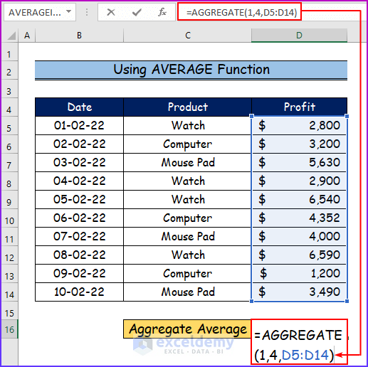
- Finally, you will see the following outcome of the AVERAGE function under the AGGREGATE function.

Read More: How to Use Conditional AGGREGATE Function in Excel
2. Inserting SUM Function
Here, you will see the sum of all the profits in the data set by using the AGGREGATE function. You may follow the steps below here.
Steps:
- Firstly, choose the D16 cell.
- Then, for inserting the SUM function, we will choose 9 for the function_num argument.
- After that, apply the following formula below here.
=AGGREGATE(9,4,D5:D14)- Then, press ENTER.
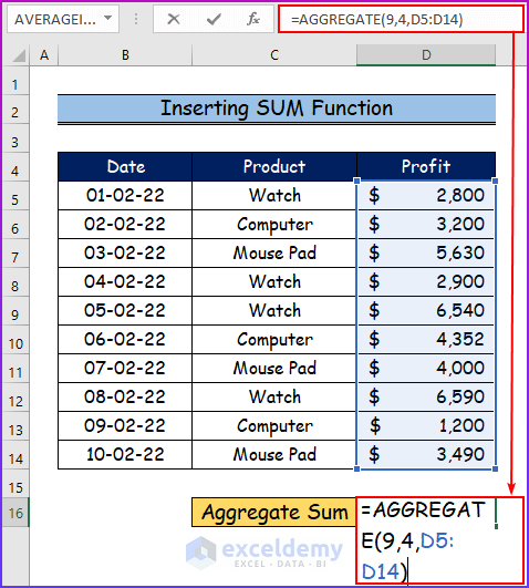
- Consequently, you will see the final result of the SUM function under the AGGREGATE function.

3. Utilizing Power Query to Aggregate Data in Excel
An application for preparing and transforming data is called Power Query. With Power Query, you may perform transformations to data obtained from sources using a Power Query Editor and a graphical user interface. You may import data from a variety of sources, clean it up, convert it, and then reshape it to suit your needs using Power Query, a business intelligence tool provided by Microsoft Excel. This allows you to create a query just once and reuse it at a later time by simply refreshing it. The best method for combining data from numerous sources is to use Excel Power Query.
Steps:
- Firstly, go to the Data tab.
- Secondly, click on the From Table/Range option from the Get & Transform Data group.
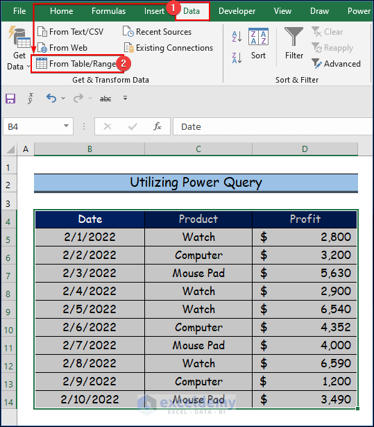
- Then, click OK.

- Here, the Power Query Editor will open.
- Then, select the Group By option here.

- Here, you will then be presented with a new window where you can choose which columns to the group.
- Afterward, select the “Advanced” option if you want to use the aggregate features.
- Then, we will choose all three columns of our data set to add more columns, selecting “Add grouping” from the menu below.
- Finally, simply enter a name in the “New column name” as the Result field to aggregate the data according to your computation preference.

- Therefore, this is how you can aggregate data from any column by adding a new column.

Download Practice Workbook
You may download the following Excel workbook for better understanding and practice it by yourself.
Conclusion
In this article, we’ve covered 3 handy methods of how to aggregate data in Excel. We sincerely hope you enjoyed and learned a lot from this article. If you have any questions, comments, or recommendations, kindly leave them in the comment section below.
Related Articles
- How to Aggregate COUNTIF in Excel
- How to Use Excel AGGREGATE Function with Multiple Criteria
- AGGREGATE Formula for Adding Serial Number in Excel
- Combining AGGREGATE with IF Function in Excel
- AGGREGATE vs SUBTOTAL in Excel
- How to Use AGGREGATE to Achieve MAX IF Behavior in Excel
- How to Combine INDEX and AGGREGATE Functions in Excel
<< Go Back to Excel AGGREGATE Function | Excel Functions | Learn Excel
Get FREE Advanced Excel Exercises with Solutions!
