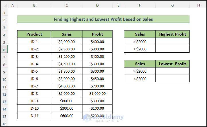
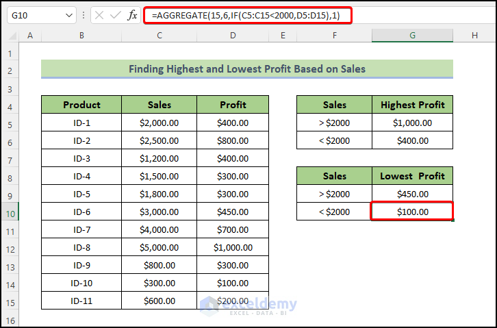
How to Combine AGGREGATE with the IF Function in Excel (4 Methods)

Method 1 – Finding the Highest and Lowest Profit Based on Sales

In this method, we’ll demonstrate how to combine the AGGREGATE and IF functions using greater than and less than criteria. For illustrative purposes, we’ll apply these functions to the following dataset, where we want to identify profits based on sales greater or less than $2000.

Combining AGGREGATE with IF Function in Excel to find highest and lowest profit

Follow these steps:

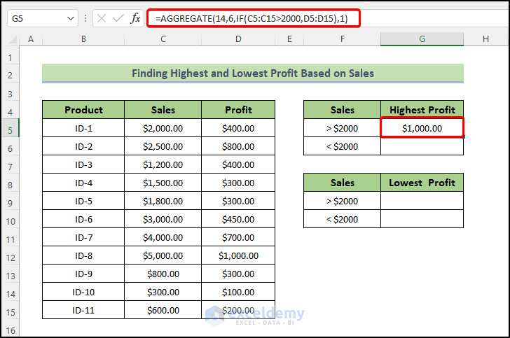
Select the cell where you want to display the result (e.g., cell G5).
Enter the following formula:

=AGGREGATE(14,6,IF(C5:C15>2000,D5:D15),1)

Press Enter.
This will give you the maximum profit based on sales greater than $2000.

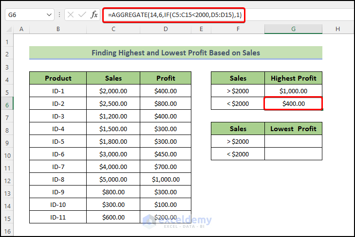
Select cell G6 and enter the following formula:

=AGGREGATE(14,6,IF(C5:C15<2000,D5:D15),1)

Press Enter.
This will give you the maximum profit based on sales less than $2000.

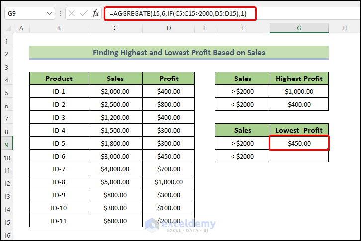
Select the cell where you want to display the result (e.g., cell G9).
Enter the following formula:

=AGGREGATE(15,6,IF(C5:C15>2000,D5:D15),1)

Press Enter.
This will give you the minimum profit based on sales greater than $2000.

Select another cell (G10) and enter the following formula:

=AGGREGATE(15,6,IF(C5:C15<2000,D5:D15),1)

Press Enter.
This will give you the lowest profit based on sales less than $2000.

How Does the Formula Work?

AGGREGATE(14, 6, IF(C5:C15 > 2000, D5:D15), 1):
- The IF function checks whether the values in the range C5:C15 are greater than 2000. If true, it collects corresponding values from D5:D15.
- The AGGREGATE function then returns the largest value (1st largest) from the collected values.
- Inside the parentheses:
  - 14 represents the LARGE function.
  - 6 means we ignore error values.
  - 1 specifies the 1st largest value.
AGGREGATE(14, 6, IF(C5:C15 < 2000, D5:D15), 1):
- Similar to the previous case, but it collects smaller values based on the IF condition.
AGGREGATE(15, 6, IF(C5:C15 > 2000, D5:D15), 1):
- Collects the largest value based on sales greater than $2000.
AGGREGATE(15, 6, IF(C5:C15 < 2000, D5:D15), 1):
- Collects the smallest value based on sales less than $2000.

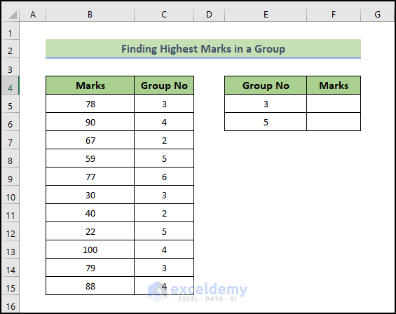
Method 2 – Finding the Highest Marks in a Group

In this method, we’ll demonstrate how to combine the AGGREGATE and IF functions in Excel. We’ll apply these functions to the following dataset to identify the highest marks based on groups not equal to 3 or 5.

Follow these steps:

Select the cell where you want to display the result (e.g., cell F5).
Enter the following formula:

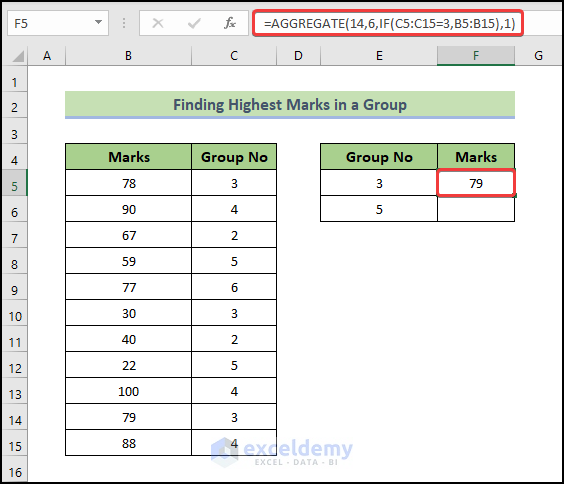
=AGGREGATE(14,6,IF(C5:C15=3,B5:B15),1)

Press Enter.
This will give you the maximum marks based on groups not equal to 3.

Select cell F6 and enter the following formula:

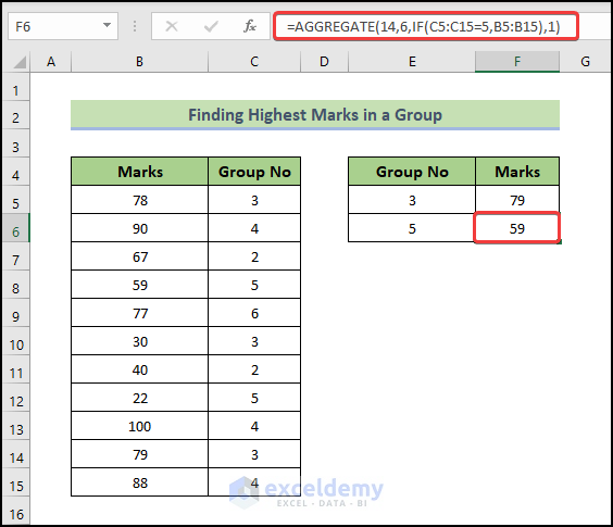
=AGGREGATE(14,6,IF(C5:C15=5,B5:B15),1)

Press Enter.
This will give you the maximum marks based on groups not equal to 5.

How Does the Formula Work?

AGGREGATE(14, 6, IF(C5:C15 = 3, B5:B15), 1):
- The IF function checks whether the values in the range C5:C15 are equal to 3. If true, it collects corresponding values from B5:B15.
- The AGGREGATE function then returns the largest value (1st largest) from the collected values.
- Inside the parentheses:
  - 14 represents the LARGE function.
  - 6 means we ignore error values.
  - 1 specifies the 1st largest value.
AGGREGATE(14, 6, IF(C5:C15 = 5, B5:B15), 1):
- Similar to the previous case, but it collects larger values based on the IF condition.

Read More: How to Aggregate Data in Excel

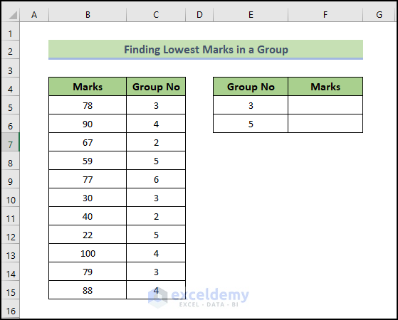
Method 3 – Finding the Lowest Marks in a Group

In this method, we’ll illustrate how to find the lowest marks based on groups not equal to 3 or 5.

Follow these steps:

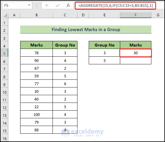
Select the cell where you want to display the result (e.g., cell F5).
Enter the following formula:

=AGGREGATE(15,6,IF(C5:C15=3,B5:B15),1)

Press Enter.
This will give you the minimum marks based on groups not equal to 3.

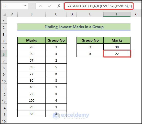
Select cell F6 and enter the following formula:

=AGGREGATE(15,6,IF(C5:C15=5,B5:B15),1)

Press Enter.
This will give you the minimum marks based on groups not equal to 5.

How Does the Formula Work?

AGGREGATE(15, 6, IF(C5:C15 = 3, B5:B15), 1):
- The IF function checks whether the values in the range C5:C15 are equal to 3. If true, it collects corresponding values from B5:B15.
- The AGGREGATE function then returns the smallest value (1st smallest) from the collected values.
- Inside the parentheses:
  - 15 represents the SMALL function.
  - 6 means we ignore error values.
  - 1 specifies the 1st smallest value.
AGGREGATE(15, 6, IF(C5:C15 = 5, B5:B15), 1):
- Similar to the previous case, but it collects smaller values based on the IF condition.

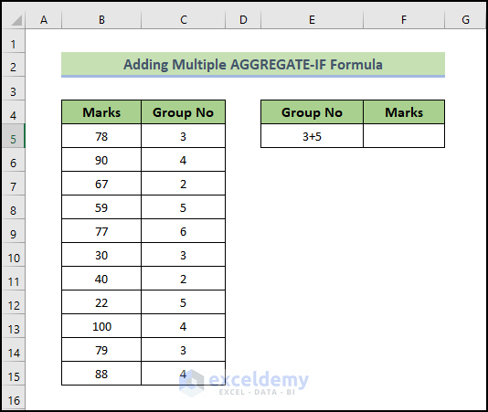
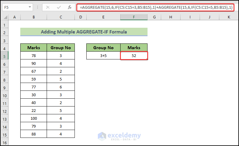
Method 4 – Adding Multiple AGGREGATE-IF Formulas

Let’s break down the steps for combining multiple AGGREGATE-IF formulas in Excel to find the lowest marks based on groups not equal to 3 and 5.

Follow these steps:

Select the cell where you want to display the result (e.g., cell F5).
Enter the following formula:

=AGGREGATE(15,6,IF(C5:C15=3,B5:B15),1)+AGGREGATE(15,6,IF(C5:C15=5,B5:B15),1)

Press Enter.
This will give you the minimum marks based on the group not equal to 3 and 5.

How Does the Formula Work?

Formula: AGGREGATE(15,6,IF(C5:C15=3,B5:B15),1)+AGGREGATE(15,6,IF(C5:C15=5,B5:B15),1)

- AGGREGATE(15, 6, IF(C5:C15 = 3, B5:B15), 1):
  - The IF function checks whether the values in the range C5:C15 are equal to 3. If true, it collects corresponding values from B5:B15.
  - The AGGREGATE function then returns the smallest value (1st smallest) from the collected values.
  - Inside the parentheses:
    - 15 represents the SMALL function.
    - 6 means we ignore error values.
    - 1 specifies the 1st smallest value.
- AGGREGATE(15, 6, IF(C5:C15 = 5, B5:B15), 1):
  - Similar to the previous case, but it collects smaller values based on the IF condition.
In the final stage, the sum of both AGGREGATE functions gives the desired output (in this case, 52).