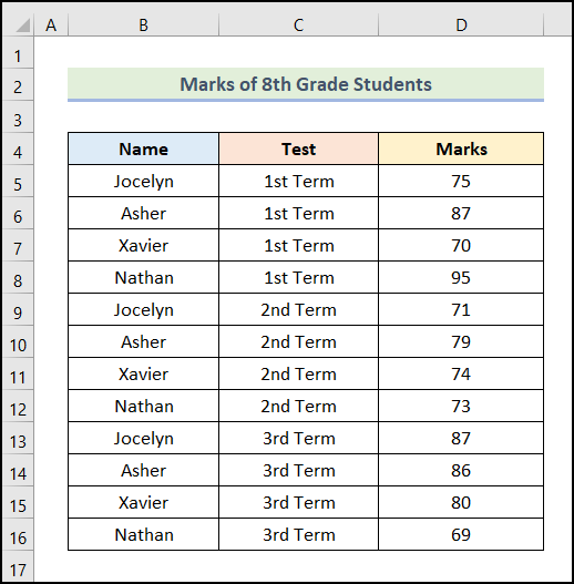
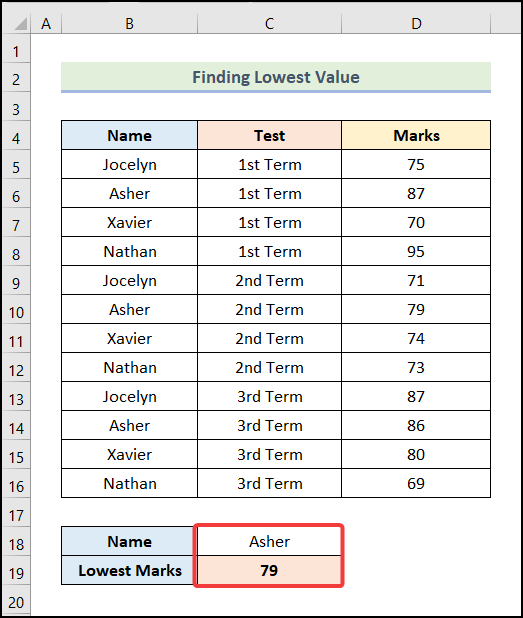
We have Marks of 8th Grade Students as our dataset. This dataset contains Marks from three terms for four Students.
Method 1 – Using the AGGREGATE Function to Find the Lowest Value
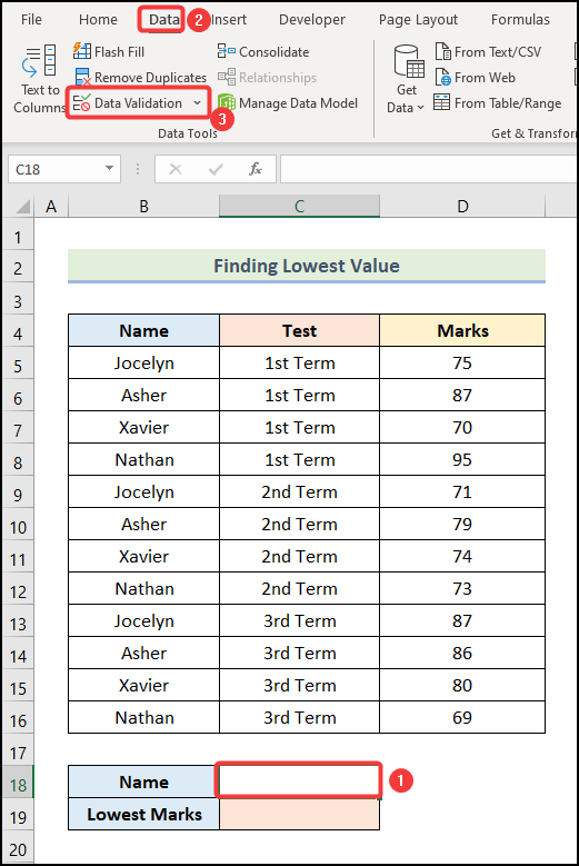
Step 1 – Create a Drop-down Button to Select the Name
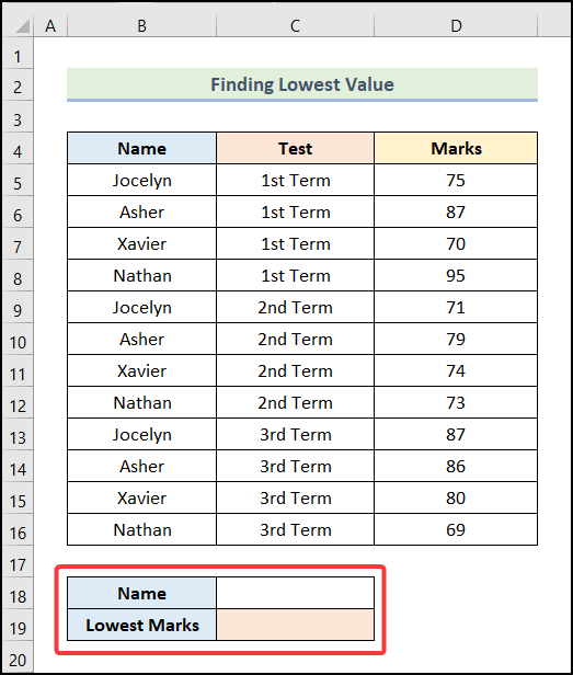
- Create a table in your worksheet as shown in the following image.
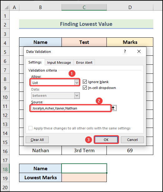
- Select the cell where you want to display the Name. We selected cell C18.
- Go to the Data tab.
- Select the Data Validation option from the Data Tools group.
The Data Validation dialog box will open on your worksheet.
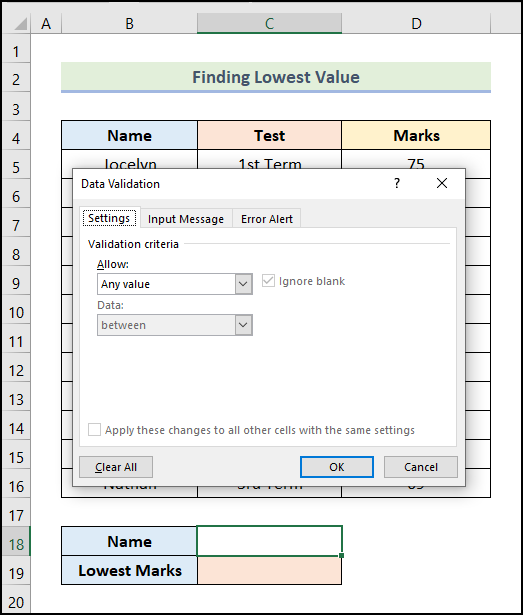
- Select the List option.
- In the Source field, type the Names of the 4 students with a comma as a separator between the Names.
- Click on OK.
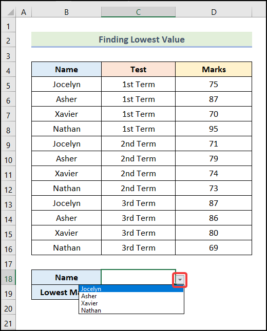
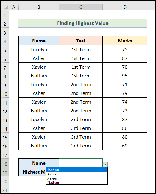
- The drop-down button will be added for cell C18. You will get the list of Names shown in the image below after clicking on the drop-down button.
Step 2 – Apply AGGREGATE Function to Find Lowest Value
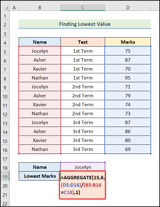
- Enter the following formula in cell C19.
=AGGREGATE(15,6,(D5:D16)/(B5:B16=C18),1)Here, the range of cells D5:D16 refers to the cells of the Marks column, the range B5:B16 represents the cells of the Name column, and the cell C18 indicates the selected Name from the drop-down list.
Formula Breakdown
- AGGREGATE(15,6,(D5:D16)/(B5:B16=C18),1) → It returns a value based on the specified function and conditions.
- 15 → It is the function_num argument. By this number, the SMALL function of Excel is specified.
- 6 → This refers to the options argument. This number represents the Ignore error values option.
- (D5:D16)/(B5:B16=C18) → It is the array argument.
- Output → {75;#DIV/0!;#DIV/0!;#DIV/0!;71;#DIV/0!;#DIV/0!;#DIV/0!;87;#DIV/0!;#DIV/0!;#DIV/0!}
- 1 → This is the [k] argument. It is an optional argument.
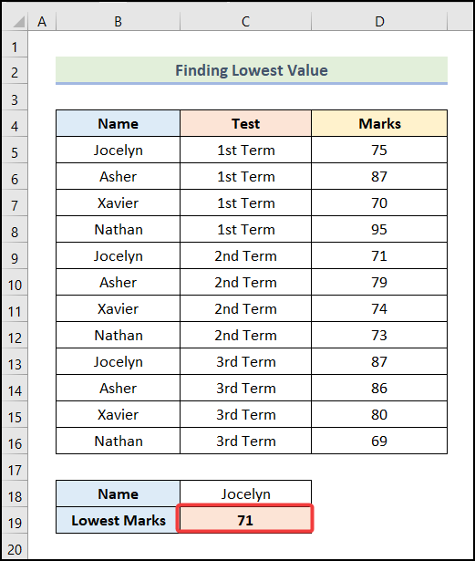
- Output → 71.
- Hit Enter.
We will get the Lowest Marks of Jocelyn.
You can also choose a different Name from the drop-down button, and your output will be adjusted automatically.
Read More: How to Use Excel AGGREGATE Function with Multiple Criteria
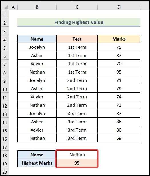
Method 2 – Utilizing the AGGREGATE Function to Find the Highest Value
Steps:
- ,Use the steps mentioned in Step 1 of Method 1 to create a drop-down button for cell C18 as shown in the image below.
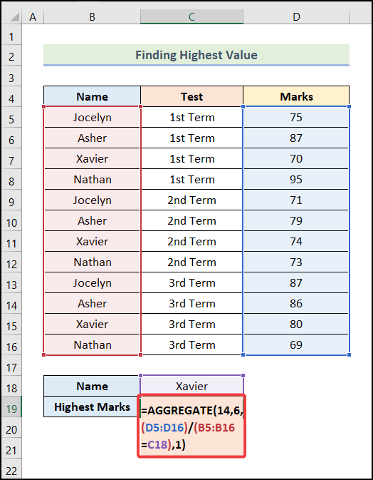
- Use the following formula in cell C19.
=AGGREGATE(14,6,(D5:D16)/(B5:B16=C18),1)Formula Breakdown
- AGGREGATE(14,6,(D5:D16)/(B5:B16=C18),1) → It gives a value based on the specified function and conditions.
- 14 → It is the function_num argument. By this number, the LARGE function of Excel is declared.
- 6 → This refers to the options argument. This number represents the Ignore error values option.
- (D5:D16)/(B5:B16=C18) → It is the array argument.
- Output → {#DIV/0!;#DIV/0!;70;#DIV/0!;#DIV/0!;#DIV/0!;74;#DIV/0!;#DIV/0!;#DIV/0!;80;#DIV/0!}
- 1 → This is the [k] argument. It is an optional argument.
- Output → 80.
- Hit Enter.
Here are the results.
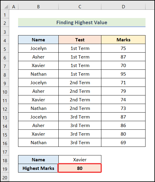
You can choose a different Name from the drop-down list and the output will change accordingly.
Exploring Some Excel Functions to Aggregate Data Based on Condition
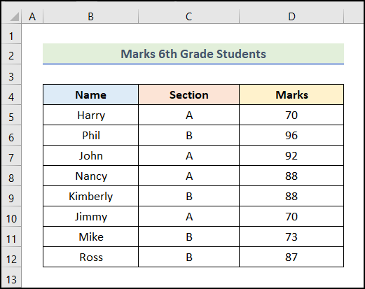
There are some functions in Excel by which we can replicate the function of the conditional AGGREGATE function. Among them, the SUMIF and the COUNTIF functions are the most common ones. We have Marks of 6th Grade Students of two Sections as our dataset.
Example 1 – SUMIF Function to Aggregate Data
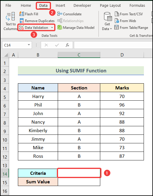
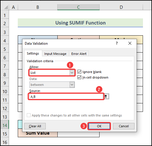
Step 1 – Create a Drop-down Button to Select the Section
- Create a table as shown in the following picture.
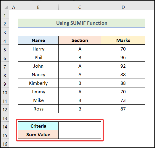
- Select the cell where you want to display the Section. We selected cell C14.
- Go to the Data tab.
- Click on the Data Validation option from the Data Tools group.
- In the Data Validation dialog box, choose the List option.
- In the field for Source, type the Name of the Sections as shown in the following picture.
- Click on OK.
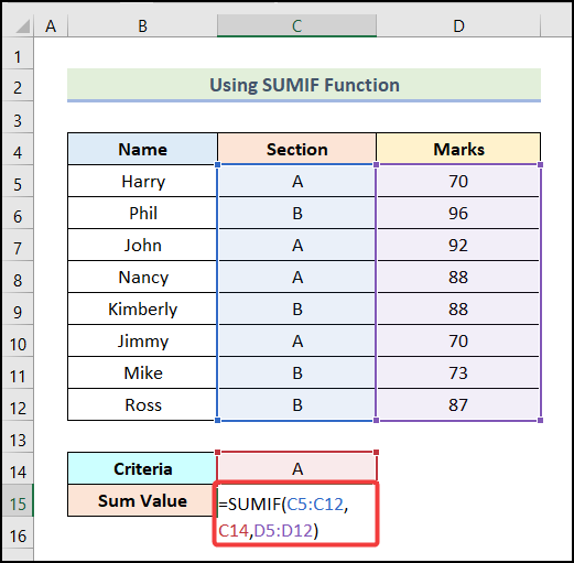
Step 2 – Apply the SUMIF Function to Calculate the Sum Value
- Enter the following formula in cell C15.
=SUMIF(C5:C12,C14,D5:D12)Here, the range of cell C5:C12 represents the cells of the Section column, range D5:D12 refers to the cells of the Marks column, and cell C14 indicates the selected Section. Now, the SUMIF function will return the sum from the sum_range D5:D12 depending upon the criteria C14 from the criteria range C5:C12.
- Hit Enter.
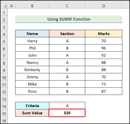
You will get the Sum Value of Marks of students in Section A as demonstrated in the image given below.
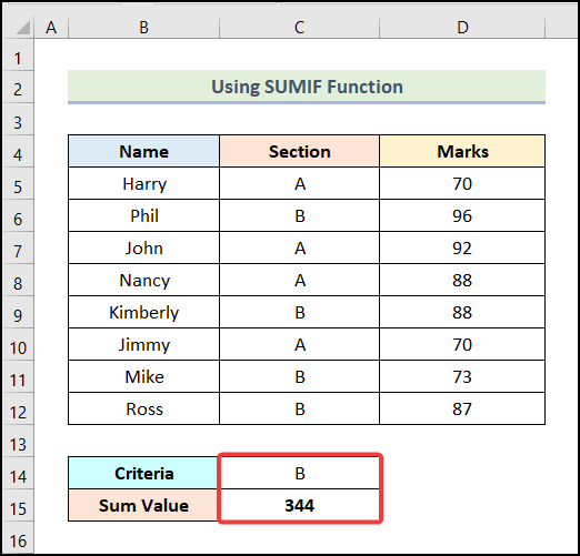
If you select Section B in the drop-down list, the Sum Value will be changed automatically.
Example 2 – Applying the COUNTIF Function to Aggregate Data Based on Condition
Steps:
- Create a table in your worksheet as shown in the following image.
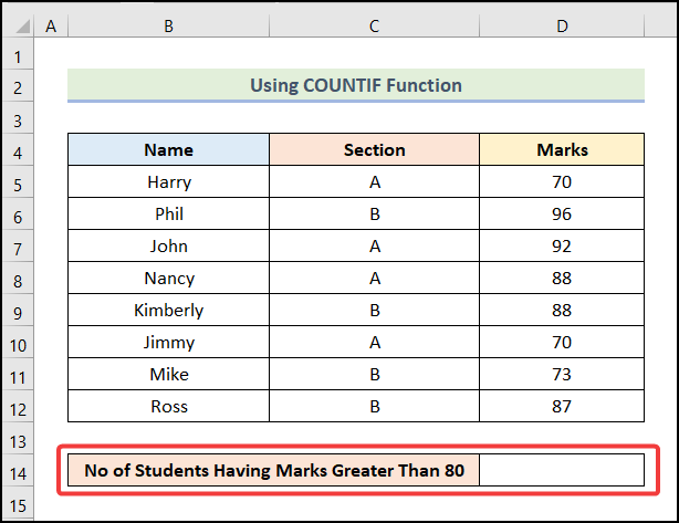
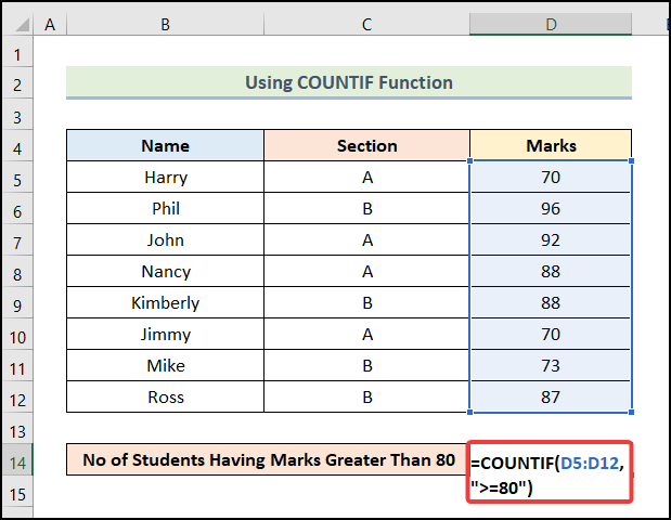
- Enter the formula given below in cell D14.
=COUNTIF(D5:D12,">=80")The COUNTIF function will return a count of cells that have a value greater or equal to 80 from the range D5:D12.
- Press Enter.
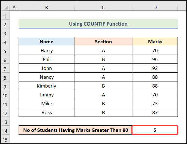
You will have the Number of Students Having Marks Greater Than 80 as demonstrated in the image below.
Read More: How to Aggregate COUNTIF in Excel
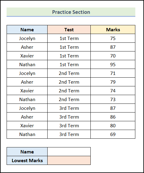
Practice Section
We have provided a Practice Section on the right side of the worksheet so you can test these methods.
Download the Practice Workbook
Related Articles
- How to Aggregate Data in Excel
- AGGREGATE Formula for Adding Serial Number in Excel
- Combining AGGREGATE with IF Function in Excel
- How to Combine INDEX and AGGREGATE Functions in Excel
- AGGREGATE vs SUBTOTAL in Excel
<< Go Back to Excel AGGREGATE Function | Excel Functions | Learn Excel
Get FREE Advanced Excel Exercises with Solutions!
