Overview of Excel LARGE Function
In the following picture, you can see the overview of the LARGE function.
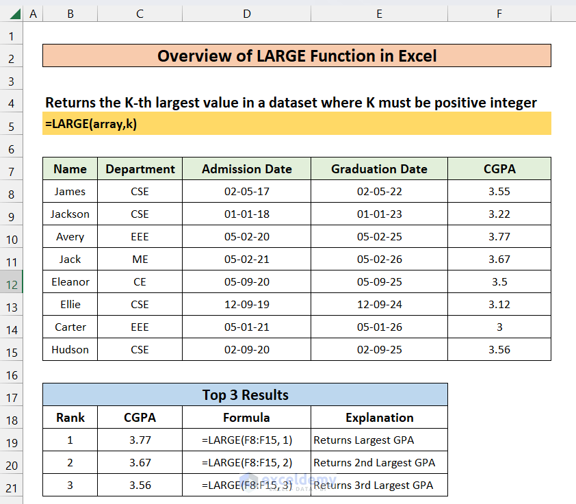
- Summary
The LARGE function returns the K-th largest value from a dataset, where K must be a positive integer.
- Syntax
=LARGE(array, k)- Arguments
| ARGUMENT | REQUIREMENT | DESCRIPTION |
|---|---|---|
| array | Required | The range of values from which you want to find the K-th largest value. |
| k | Required | An integer specifying the position (n) of the largest value. |
Note:
- K should be greater than 0.
- LARGE(array,1) returns the largest value and LARGE(array,n) returns the smallest value if there are n data points in the range.
- This function works only with numeric values, ignoring text, blank cells, and logical values.
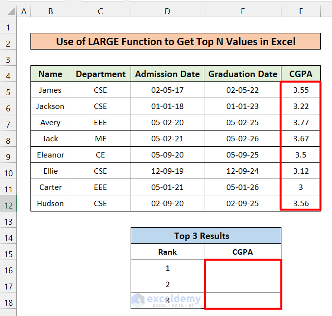
Example 1 – Top N Values Using LARGE
Suppose we have a dataset of students with their CGPA. To find the top 3 results using LARGE, follow these steps:
- Enter the formula in cell E16 and copy it down to E18:
=LARGE($F$5:$F$12, D16)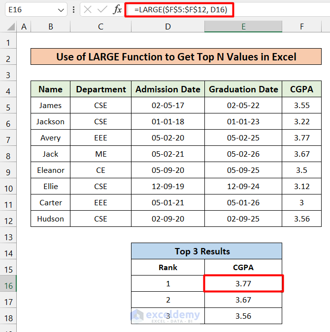
How Does the Formula Work?
- LARGE($F$5:$F$12, D16)
Here, $F$5:$F$12 is the range, and D16 specifies the position of the searching elements.
Read More: How to Find Largest Number in Excel
Example 2 – Average Largest N CGPA
To find the average CGPA of the top 4 students, combine LARGE and AVERAGE:
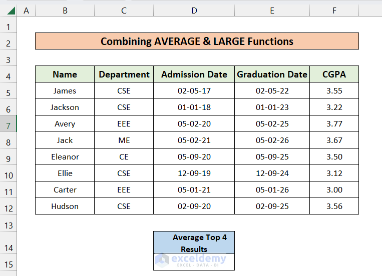
- Enter the following formula in cell D15.
=AVERAGE(LARGE(F5:F12, {1,2,3,4}))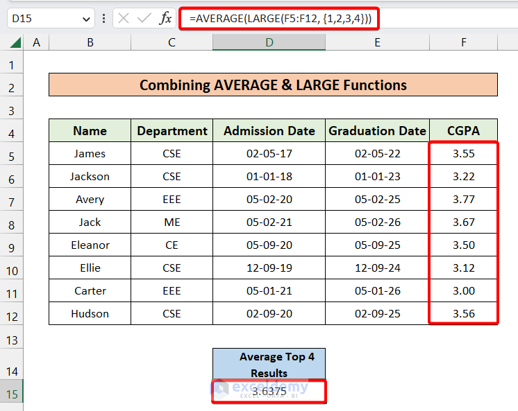
How Does the Formula Work?
- LARGE(F4:F11, {1,2,3,4})
This portion will find the top 4 largest values from the CGPA dataset. {1,2,3,4} this is used to define the top 4 values using an array argument.
- AVERAGE(LARGE(F5:F12, {1,2,3,4}))
The AVERAGE function calculates the average of the selected values.
Example 3 – Sum of Largest N CGPA
To calculate the sum of the top 4 students’ GPAs:
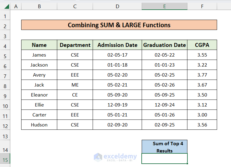
- Enter this formula in cell E15:
=SUM(LARGE(F5:F12, {1,2,3,4}))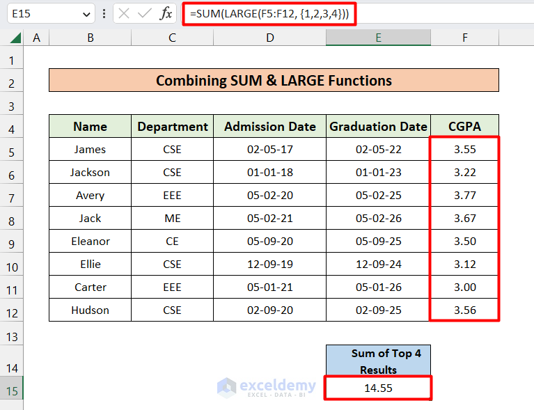
How Does the Formula Work?
- LARGE(F4:F11, {1,2,3,4})
This portion will find the top 4 largest values from the CGPA dataset. {1,2,3,4} this is used to define the top 4 values using an array argument.
- SUM(LARGE(F5:F12, {1,2,3,4}))
The SUM function returns the summation.
Example 4 – Associated Data with Largest Value
Sometimes we need associated data with the largest value. Use INDEX, MATCH, and LARGE:
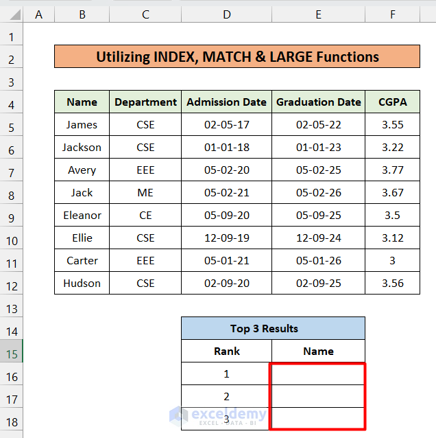
- Enter this formula in cell E16 and copy it down to E18:
=INDEX($B$5:$B$12, MATCH(LARGE($F$5:$F$12, $D16), $F$5:$F$12, 0))
This will return the student names corresponding to the largest CGPA values in column F.
How Does the Formula Work?
- LARGE($F$5:$F$12, $D16)
This portion of the formula finds the highest (D16=1) CGPA in the F5:F12 range.
- MATCH(LARGE($F$5:$F$12, $D16), $F$5:$F$12, 0)
This portion of the formula provides the row number of the top CGPA holder in the F5:F12 column.
- INDEX($B$5:$B$12, MATCH(LARGE($F$5:$F$12, $D16), $F$5:$F$12, 0))
Lastly, the INDEX function will return the associated data with the largest value from $B$5:$B$12 column.
Read More: How to Lookup Next Largest Value in Excel
Example 5 – Sorting Numbers in Descending Order
Suppose we want to sort students’ CGPA in a separate column called Sorted CGPA.
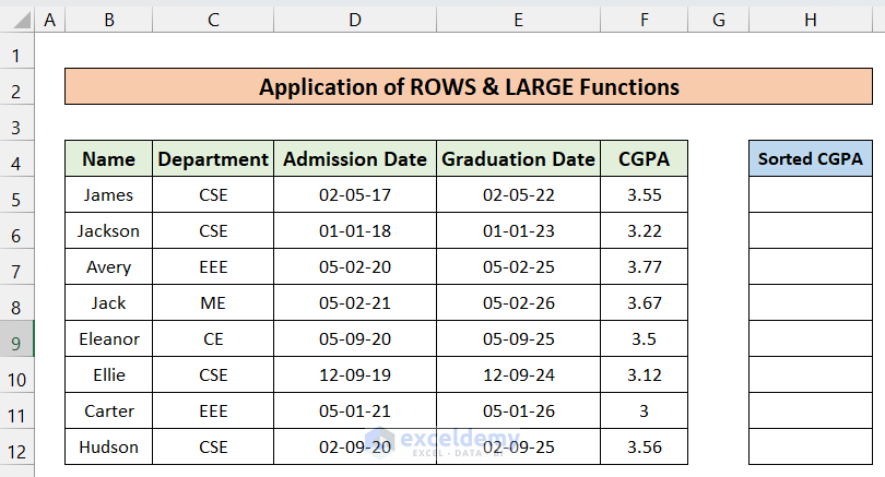
We can achieve this using the ROWS and LARGE functions. Follow these steps:
- Enter the formula in cell H5 and copy it down to H12:
=LARGE($F$5:$F$12, ROWS(F$5:F5))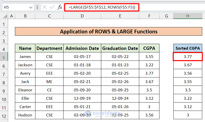
How Does the Formula Work?
- ROWS(F$5:F5)
Returns the row number within the range.
- LARGE($F$5:$F$12, ROWS(F$5:F5))
Finds the largest numbers from the $F$5:$F$12 range.
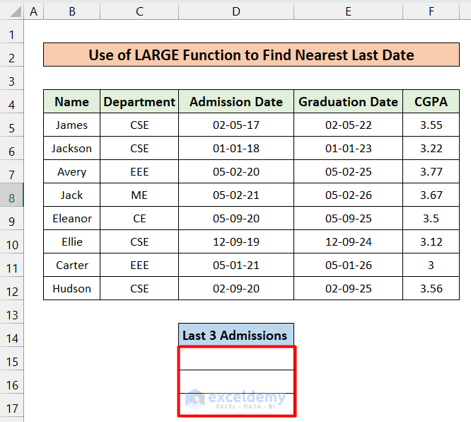
Example 6 – Finding Nearest Dates
To find the most recent admission dates for the top 3 students, use the LARGE and ROWS functions:
- Enter the formula in cell D15 and copy it down to D17:
=LARGE($D$5:$D$12, ROWS(D$5:D5))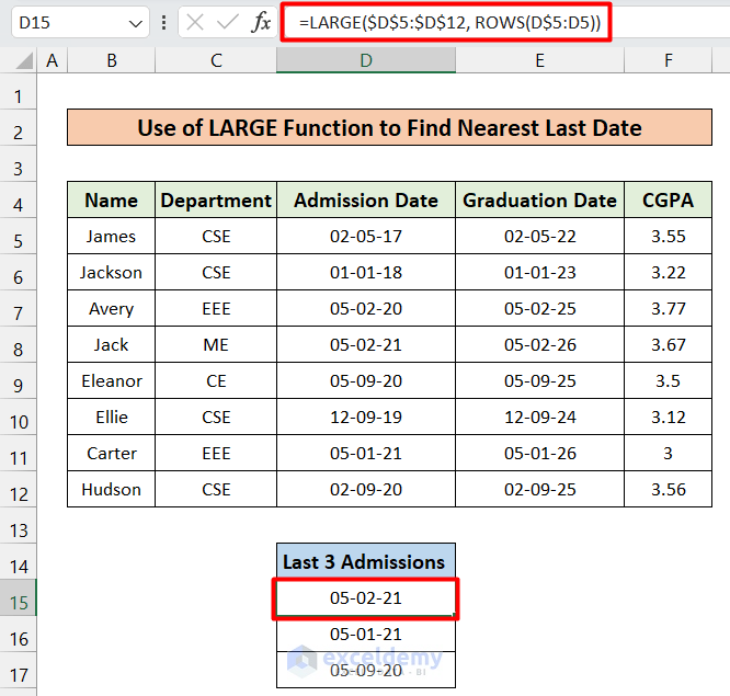
Read More: How to Find Second Largest Value with Criteria in Excel
Example 7 – Upcoming Dates Nearest to Today
Suppose today is November 9, 2022. To find the top 3 graduation dates near the current date:
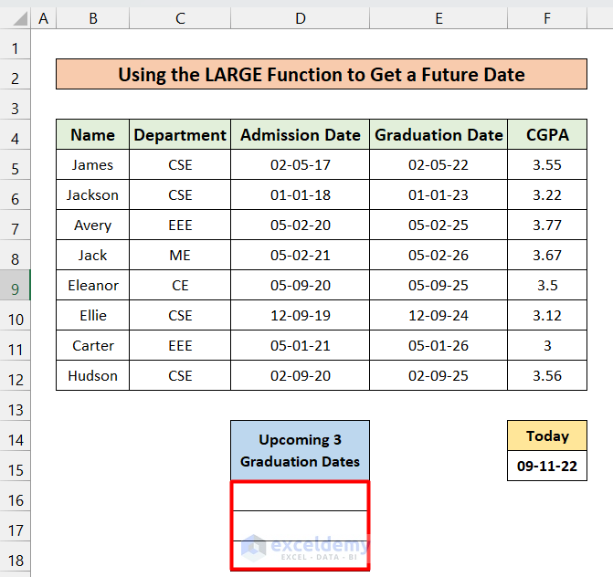
- Enter the following formulas in cells D16, D17, and D18 respectively:
=LARGE($E$5:$E$12, COUNTIF($E$5:$E$12, ">"&TODAY()))And,
=LARGE($E$5:$E$12, COUNTIF($E$5:$E$12, ">"&TODAY())-1)And,
=LARGE($E$5:$E$12, COUNTIF($E$5:$E$12, ">"&TODAY())-2)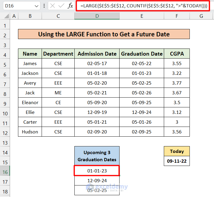
How Does the Formula Work?
- COUNTIF($E$5:$E$12, “>”&TODAY())
This part will count the number of cells using the condition. The condition is the date must be greater than today. Today’s date is found using the TODAY function. To know more about TODAY and COUNTIF functions, you can check these two articles:
- LARGE($E$5:$E$12, COUNTIF($E$5:$E$12, “>”&TODAY()))
The LARGE function is used to find the largest dates.
When Will the LARGE Function Not Work in Excel?
This LARGE function will not work under the following circumstances:
- The k value is negative.
- The k value exceeds the number of values in the array.
- The provided array is empty or lacks numeric values.
Things to Remember
| COMMON ERRORS | WHEN THEY ARE SHOWN |
|---|---|
| #NUM! | This error occurs if the array is empty or if the value of k (position) is less than or equal to 0, or greater than the number of data points. |
| #VALUE! | This error appears if the supplied k is a non-numeric value. |
Frequently Asked Questions
- Alternative Functions:
- If you want to find the largest value in a range without specifying a position, you can use the MAX function.
- Handling Duplicate Values:
- The LARGE function can handle arrays with duplicate values. It treats duplicate values as separate entries and retrieves the kth largest value accordingly.
- Using LARGE Across Worksheets:
- Yes, you can use the LARGE function with a range of cells in a different worksheet. Specify the worksheet name along with the cell range. For example, use ‘Sheet2!A1:A10’ to refer to cells A1 to A10 in Sheet2.
Download Practice Workbook
You can download the practice workbook from here:
Excel LARGE Function: Knowledge Hub
<< Go Back to Excel Functions | Learn Excel
Get FREE Advanced Excel Exercises with Solutions!
