Today we will discuss the use of the LARGE function to get the associated text data of a specific numeric value in Excel. The LARGE function returns the k-th largest value of a dataset, where the integer k specifies the position of the largest numeric value in the array or range of cells of data. We can only extract numeric values using the LARGE function. However, by combining the LARGE function with some other useful functions, we can extract the associated text data of a numeric value.

How to Use Excel Large Function with Text: 3 Easy Ways
In this article, we will demonstrate how we can use the LARGE function to get the associated text data of a particular numeric value. We can use the LARGE function with the VLOOKUP function. Moreover, we can also use the LARGE function with INDEX, and MATCH functions. We can use the ROWS function along with the LARGE function to get the associated text data of any particular numeric value as well.
Method 1: Combining LARGE and VLOOKUP Functions to Get Text Data in Excel
We can use the LARGE function with the VLOOKUP function to retrieve the associated text data of a numeric value. This method is simple and easy to use. Here in this worksheet, we have the names of multiple students, their student IDs, their GPAs (Grade Point Average), their departments, and their permanent addresses. We want to find out the names of the top 3 students with the highest GPAs.
Steps:
- Select the cell where you want to put the name of the student. We are selecting cell E15, where we want to see the name of the student who has the highest GPA.

- Enter the formula in cell E15.
=VLOOKUP(LARGE($C$5:$C$11,D15),$C$5:$F$11,2,0)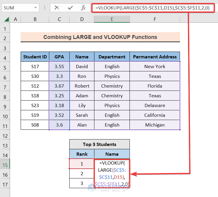
How Does the Formula Work?
- LARGE($C$5:$C$11,D15), this portion of the formula finds the highest (D15=1) GPA in range C5:C11.
- VLOOKUP(LARGE($C$5:$C$11,D15),$C$5:$F$11,2,0), the VLOOKUP function looks for the highest GPA value in the range C5:F11.
- Then, it returns the exact match of the text data corresponding to the highest GPA value from column no 2 (Name) of the selected range (C5:F11).
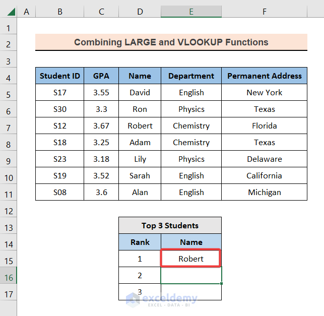
- Press Enter and you will see the name of the student with the highest GPA. In this dataset, Robert has the highest GPA (3.67) among all the students. That’s why his name has appeared in cell E15.
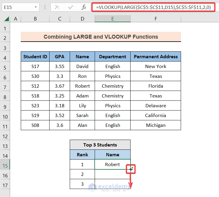
- Select cell E15 and copy the formula up to cell E17 by using the AutoFill tool.
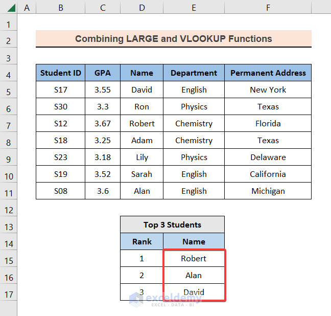
- Finally, you will have the names of the top 3 students with the highest GPAs.
Read More: How to Use LARGE Function with VLOOKUP Function in Excel
Method 2: Nesting LARGE Function with INDEX, and MATCH Functions to Extract Text Data in Excel
We can use a combination of the LARGE, INDEX, and MATCH functions to extract the associated text data of a numeric value. The INDEX and MATCH functions are the perfect alternative to the VLOOKUP function. The VLOOKUP function has some limitations. The biggest drawback of the VLOOKUP function is, that it can extract data only from the columns that are situated on the right-hand side of the look-up value. Also, the lookup value has to be on the leftmost column of the selected range of cells. The best way to overcome this limitation is to use the INDEX and MATCH functions. We will use the same dataset as Method 1. Simply follow the steps below:
Steps:
- First, select the cell where you want to put the name of the student. We are selecting cell E15, where we want to see the name of the student who has the highest GPA.
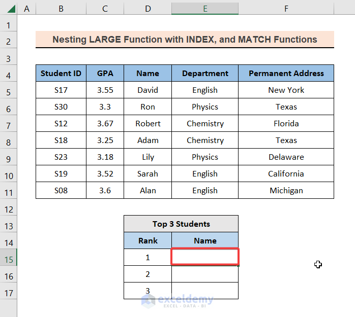
- Type the formula in cell E15.
=INDEX($D$5:$D$11,MATCH(LARGE($C$5:$C$11,D15),$C$5:$C$11,0),0)
How Does the Formula Work?
- LARGE($C$5:$C$11,D15), this portion of the formula finds the highest (D15=1) GPA in range C5:C11.
- MATCH(LARGE($C$5:$C$11,D15),$C$5:$C$11,0), this portion of the formula provides the row of the top GPA holder in range C5:C11.
- INDEX($D$5:$D$11,MATCH(LARGE($C$5:$C$11,D15),$C$5:$C$11,0),0), the INDEX function will return the exact match of the associated text data with the largest value from range D5:D11.
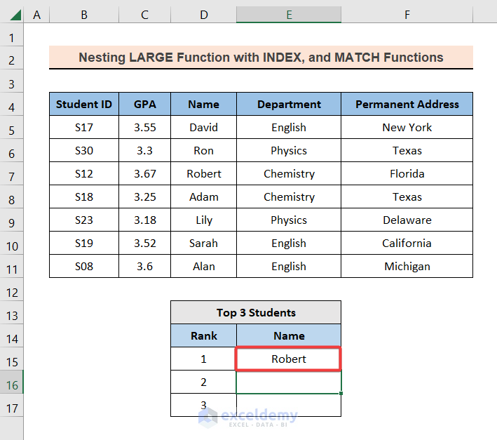
- After that, press Enter and you will see the name of the student with the highest GPA.
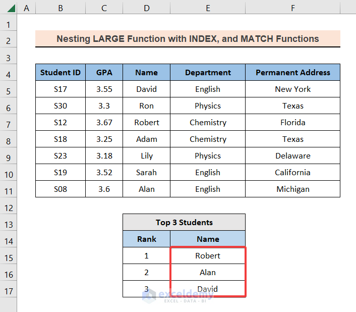
- Select cell E15 and copy down the formula up to cell E17.

- Finally, you will have the names of the top 3 students with the highest GPAs.
Read More: How to Use Excel LARGE Function with Criteria
Method 3: Combining LARGE Function with INDEX, MATCH, and ROWS Functions to Sort Text Data in Descending Order
We can sort numbers in descending order by using the LARGE function with the ROWS function and subsequently sort the associated text data of those numbers. Here in the dataset, the names of the students are not sorted according to their GPAs. We can sort the names in such a way that the highest GPA holder gets the topmost position and the lowest GPA holder gets the bottommost position. In short, we will sort the names of all the students with their GPAs in descending order. Simply follow the steps below:
Steps:
- To begin, select the cell to start the order. We are selecting cell H5.
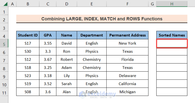
- Next, enter the formula in cell H5.
=INDEX($D$5:$D$11,MATCH(LARGE($C$5:$C$11,ROWS(C$5:$C5)),$C$5:$C$11,0),0)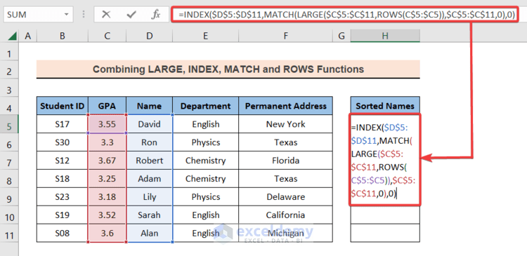
How Does the Formula Work?
- ROWS(C$5:C5), this portion of the formula returns the row number of the reference.
- LARGE($C$5:$C$11, ROWS(C$5:C5)), the LARGE function finds all the large numbers according to the row serial from range C5:C11.
- MATCH(LARGE($C$5:$C$11,ROWS(C$5:$C5)),$C$5:$C$11,0), moreover, this portion of the formula provides the row of the descending GPA holder in the range C5:C11.
- INDEX($D$5:$D$11,MATCH(LARGE($C$5:$C$11,ROWS(C$5:$C5)),$C$5:$C$11,0),0), finally, the INDEX function will return the exact match of the associated text data with the largest value from the range D5:D11.
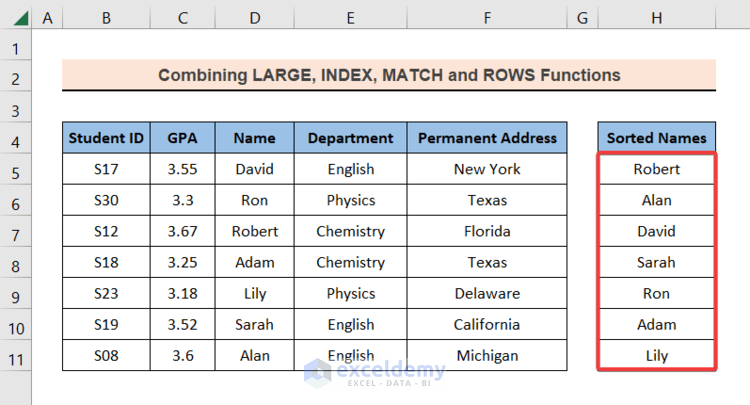
- Now, press Enter and you will see the name of the student.

- Copy down the formula up to H11 with the AutoFill tool and you will see the list of students in H5:H11 with their GPAs in descending order.
Things to Remember
The LARGE function will not work if any of the following circumstances occur:
- If the second argument (k value) of the LARGE function is a negative number.
- If the k value is higher than the number of rows in the specified range.
- The selected array is empty or doesn’t include a single numeric value.
Download Practice Book
You can download this practice workbook while going through this article.
Conclusion
In this article, we have demonstrated how to use the LARGE function along with some other useful functions to retrieve the associated text data in Excel. This article will allow users to use Excel more efficiently and effectively. If you have any questions regarding this essay, feel free to let us know in the comments. Also, if you want to see more Excel content like this, please visit our website and unlock a great resource for Excel-related content.
Related Articles
- How to Find Largest Number in Excel
- How to Use Excel LARGE Function in Multiple Ranges
- How to Use Excel LARGE Function with Duplicates in Excel
- How to Lookup Next Largest Value in Excel
- How to Use VBA Large Function in Excel
- How to Find Second Largest Value with Criteria In Excel
- How to Use LARGE and SMALL Function in Excel
<< Go Back to Excel LARGE Function | Excel Functions | Learn Excel

