Method 1 – Using LARGE Function
The LARGE function can return the largest number from a list of numbers after we sorted it in descending order. Let us see how to apply this function to find the second largest value with criteria.
Steps:
- Go to cell F7 and insert the following formula.
=LARGE(IF(C4:D4=F5,C5:D10),2)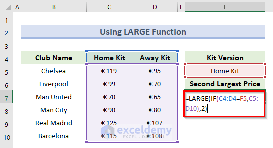
- Press Enter and this will calculate the second largest Home Kit price in cell F7.
How Does the Formula Work?
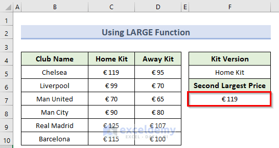
- IF(C4:D4=F5,C5:D10): This portion returns an array of the cell values and FALSE cell values.
- =LARGE(IF(C4:D4=F5,C5:D10),2): This part of the formula returns the final value of 119.
Read More: How to Find Largest Number in Excel
Method 2 – Applying AGGREGATE Function
The AGGREGATE function gives us the ability to perform aggregate calculations like COUNT, AVERAGE, MAX, etc. This function also ignores any hidden rows or errors. We will use this function to find the second-largest value with specific criteria.
Steps:
- Enter the following formula in F7.
=AGGREGATE(14,6,(C5:D10)/(C4:D4=F5),2)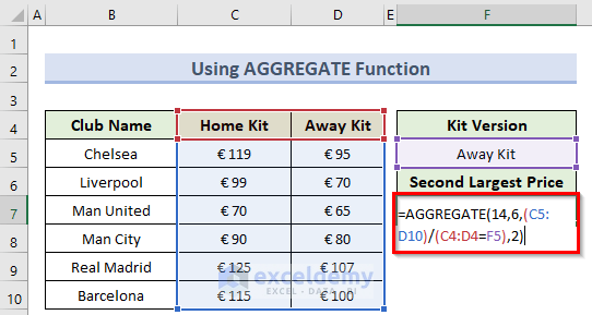
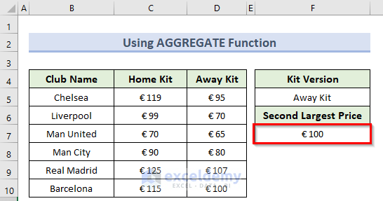
- Press the Enter key and you will get the second-largest Away Kit.
Method 3 – Utilizing SUMPRODUCT Function
The SUMPRODUCT function first multiplies the range of values and gives the sum of those multiplications. We can use this function along with the LARGE function to find the second largest value with criteria.
Steps:
- Enter the following formula in F7.
=SUMPRODUCT(LARGE((B5:B10=F5)*(C5:D10),2))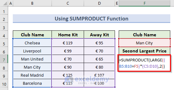
- Press the Enter key and you will find the second largest price value for the Man City kit in cell C10.
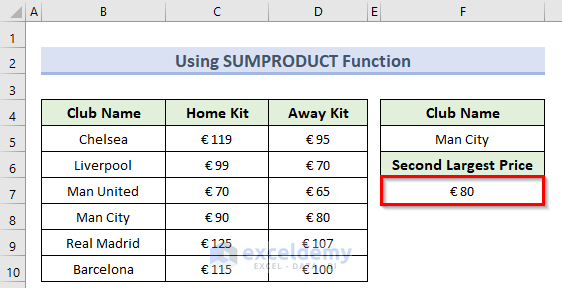
How Does the Formula Work?
- (B5:B10=F5)*(C5:D10): This portion of the formula returns an array of values that are the highest in the list and other values as 0.
- LARGE((B5:B10=F5)*(C5:D10),2): This portion gives the value 80 as the second largest value.
- =SUMPRODUCT(LARGE((B5:B10=F5)*(C5:D10),2)): This part gives back the final value which is 80 in this case.
Read More: How to Lookup Next Largest Value in Excel
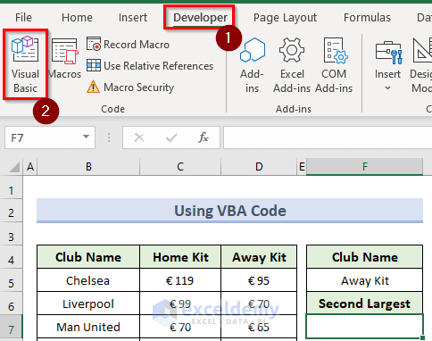
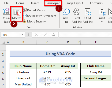
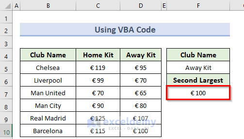
Method 4 – Using VBA Code
Steps:
- Go to the Developer tab and select Visual Basic.
- Select Insert in the VBA window and click on Module.
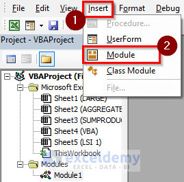
- Enter the following code in the new window.
Sub SecondLargest()
Range("F7").FormulaArray = "=LARGE(IF(C4:D4=F5,C5:D12),2)"
End Sub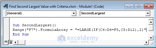
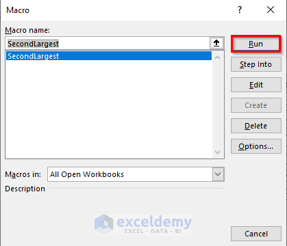
- Open the macros from the Developer tab by clicking on Macros.
- From the Macro window, select the macro named SecondLargest and click Run.
- The VBA code will calculate the second-highest value from all the away kits in cell F7.
How to Find Top 5 Values and Names with Criteria in Excel
Steps:
- Enter the following formula in cell E5.
=LARGE($C$5:$C$10,ROWS($E$5:$E5))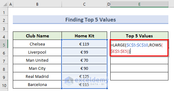
- Press the Enter key and copy this formula to the remaining cells using the Fill Handle tool.
- This will find the top 5 values for the home kits.
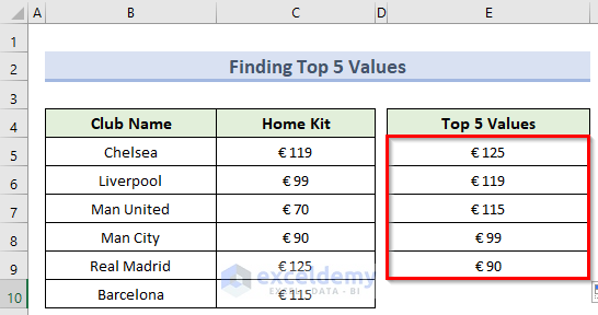
How Does the Formula Work?
- ROWS($E$5:$E5): This portion gives the value of 1.
- =LARGE($C$5:$C$10,ROWS($E$5:$E5)): This portion returns the final value which is the top 5 home kit prices.
Things to Remember
- You can use the ALT + F11 shortcut to open the VBA window and ALT + F8 to open the Macros window.
- Note that the LARGE function ignores cells that are empty or contain TRUE or FALSE values in them.
- If there is no numeric value, this function might return the #NUM! error.
Download Practice Workbook
Related Articles
- How to Use Excel LARGE Function with Criteria
- How to Use Excel LARGE Function with Duplicates in Excel
- How to Use Excel Large Function with Text
- How to Use LARGE Function with VLOOKUP Function in Excel
- How to Use Excel Large Function in Multiple Ranges
- How to Use LARGE and SMALL Function in Excel
<< Go Back to Excel LARGE Function | Excel Functions | Learn Excel
Get FREE Advanced Excel Exercises with Solutions!

I have a range of cells containing,
12,
12,
12,
12,
11,
10,
9,
1,
0.
I want a return of second highest row2 (12) in formula
Hi D V V NARAYANARAJU,
Thank you very much for reading our articles.
In your query, you wanted to know how to return the second highest value which is 12 located at row 2 using the formula.
You can use the following formula:
=LARGE($B$5:$B$13,2)We have inserted the values in the range B5:B13.
In return, we get 12 which indicates cell B6 which is the 2nd row of the range.
If you have further queries regarding this topic, then inform us.
Regards
Alok
ExcelDemy