If you want to find the 3rd most expensive smartphone from a list of smartphones, or you’re searching to solve a problem like this, you’re on the right page. Excel offers functions named LARGE and SMALL for this purpose. In this article, I’m going to share how to use LARGE and SMALL functions in Excel with suitable examples and explain them.
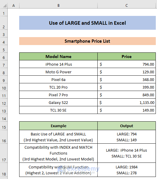
You will get a glimpse of our work in this article from this image.
How to Use LARGE and SMALL Function in Excel: 3 Examples
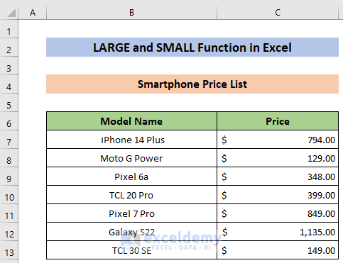
In this example, we have the price list of various models of smartphones. We want to find the k-th largest (say 3rd most expensive for example) or smallest (say 2nd least expensive for example) smartphone from this list.
- Our dataset looks like this.
1. Basic Use of LARGE and SMALL Functions in Excel
In this section, we will show how to use the LARGE and SMALL functions typically. From our dataset, we will find the 3rd highest and 2nd lowest values.
Let’s start with finding the 3rd highest value.
- Type the following formula in cell B15 and hit ENTER.
=LARGE(C7:C13,3)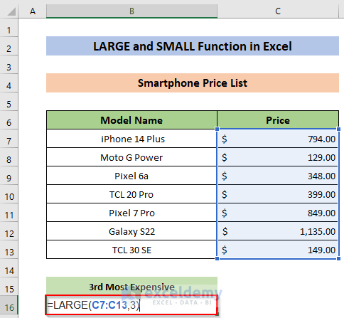
- The output looks like below.
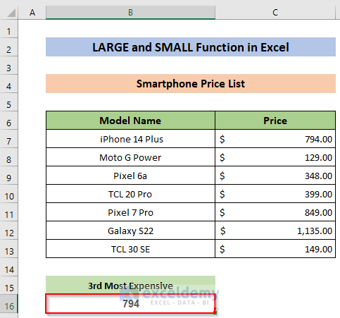
So, the price of the 3rd most expensive smartphone is $794.
- For the 2nd least value, type the following formula in cell B19.
=SMALL(C7:C13,2)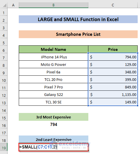
- The output looks like this.
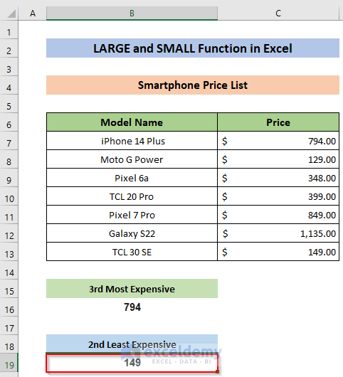
So, the price of the 2nd least expensive smartphone is $149.
Read More: How to Use VBA Large Function in Excel
2. Use of LARGE or SMALL Functions for Compatibility with INDEX and MATCH
If we want to get the Model Name of the k-th most expensive smartphone, we need to use a combination of INDEX, MATCH, and LARGE functions.
To know the details of INDEX and MATCH functions, you may check these linked articles.
Steps:
Let’s find out the 3rd most expensive smartphone’s Model Name.
- Type the following formula in cell C16 and hit ENTER.
=INDEX(B7:B13, MATCH((LARGE(C7:C13, 3)), C7:C13, 0))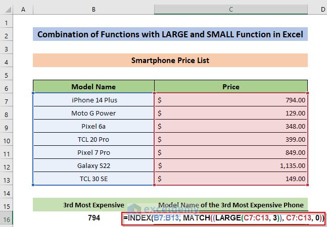
- The output looks like this.
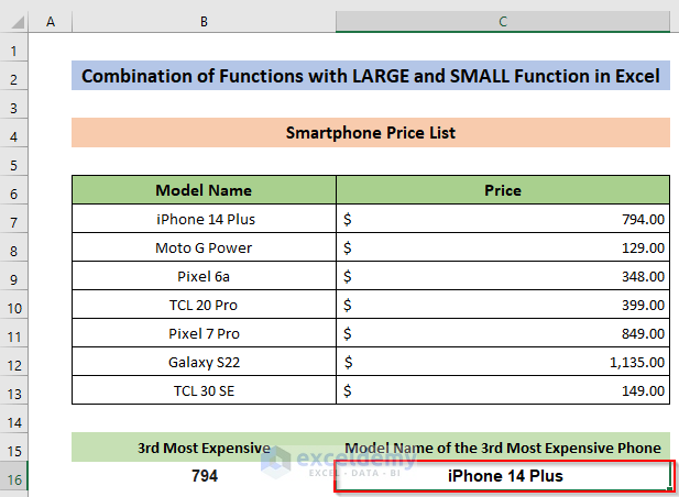
So the output says that the third most expensive phone in our list is the iPhone 14 Plus.
Formula Breakdown
The entire formula is:
=INDEX(B7:B13, MATCH(LARGE(C7:C13, 3)), C7:C13, 0))
- LARGE(C7:C13, 3): Here the LARGE function is looking for the 3rd largest value in range C7:C13.
Output: 794
- MATCH(794, C7:C13, 0): Here MATCH is looking for the row number among the range C7:C11 that contains the value 794.
Output: 1
- INDEX($B$7:$B$13,1): INDEX function takes row number 1 as input and returns the corresponding value from range $B$7:$B$13.
Output: iPhone 14 Plus - So the final output is: iPhone 14 Plus
Let’s find out the 2nd least expensive smartphone’s Model Name.
- Type the following formula in cell C19 and hit ENTER.
=INDEX(B7:B13, MATCH((SMALL(C7:C13, 2)), C7:C13, 0))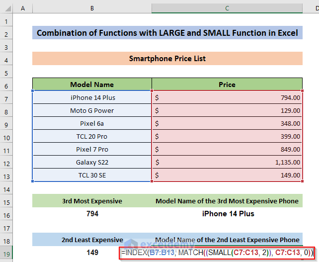
- The output looks like this.
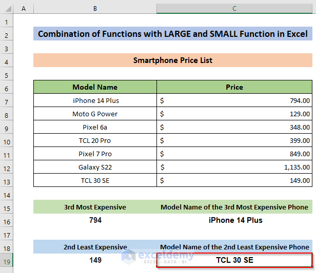
So the output says that the 2nd least expensive phone is TCL 30 SE.
The formula breakdown of this SMALL segment is quite similar to the just mentioned LARGE segment.
Read More: How to Find Largest Number in Excel
3. Use of LARGE and SMALL with Excel SUM Function
If we want to get the sum of the prices of the first two most expensive smartphones, we may use the SUM function along with the LARGE function.
Steps:
- Type the following formula in cell B16 and hit ENTER.
=SUM(LARGE(B3:B10,{1,2}))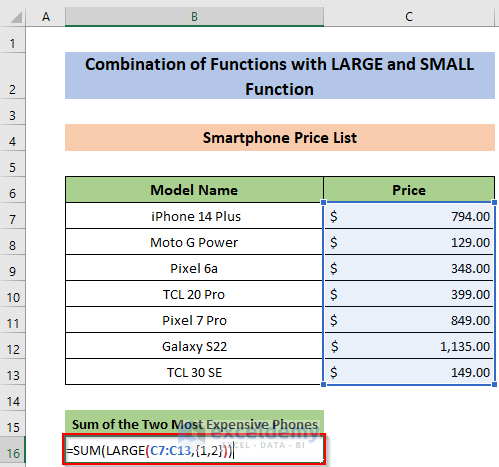
Here, {1,2} indicates the k value. At first, k takes the value 1 and performs the calculation, then it takes the value 2 and does the calculation.
- The output of the formula looks like this.
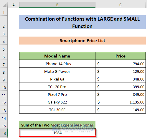
The sum of the first two most expensive smartphones is $1984.
Now, if we want to get the summation of the two least expensive phones, we need to follow these steps.
- Type the following formula in cell B19 and hit ENTER.
=SUM(SMALL(B3:B10,{1,2}))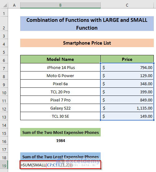
Here, {1,2} indicates the k value. At first, k takes the value 1 and does the calculation, then it takes the value 2 and does the calculation.
- The output of the formula looks like this.
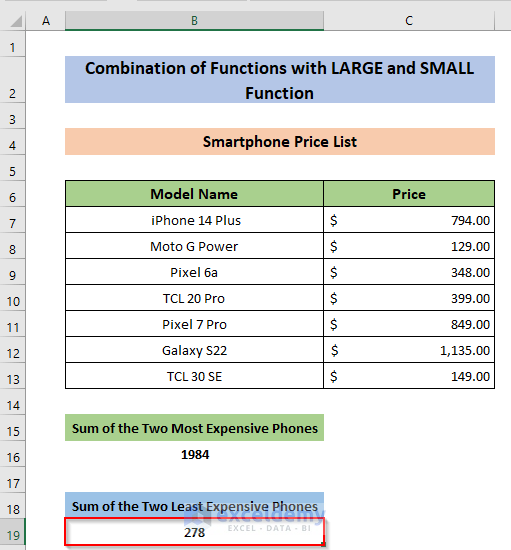
So, the sum of the first two least expensive smartphones is $278.
Read More: How to Use Excel LARGE Function with Criteria
Things to Remember
- The value of k neither can exceed the number of elements in the data array nor be zero (0) or be taken from a range of negative numbers. Also, the array cannot be empty. If any of these happens, the LARGE and SMALL functions in Excel return #NUMBER! error.
- LARGE and SMALL functions ignore the Text type data in the array.
- If the value of k becomes 1 by any means, then the output of the LARGE and SMALL functions will be the same as the output of the MAX and MIN functions respectively.
Download Practice Workbook
You may download the Workbook and practice yourself.
Conclusion
If you’re in this segment, I thank you for your interest in this content. I’ve demonstrated the details of how to use the LARGE and SMALL functions in Excel. I hope you get the necessary solution. If you face any problem regarding this article or have any queries, please feel free to leave a comment in the comment box below, Exceldemy team will try to solve that for you. Have a good day!
Related Articles
- How to Use Excel Large Function with Text
- How to Use LARGE Function with VLOOKUP Function in Excel
- How to Use Excel LARGE Function with Duplicates in Excel
- How to Use Excel Large Function in Multiple Ranges
- How to Lookup Next Largest Value in Excel
- How to Find Second Largest Value with Criteria In Excel
<< Go Back to Excel LARGE Function | Excel Functions | Learn Excel

