This is an overview.
Method 1 – Combine the LARGE and the VLOOKUP Functions to Extract Associated Text Data in Excel
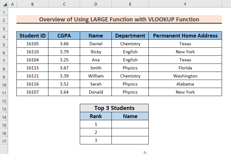
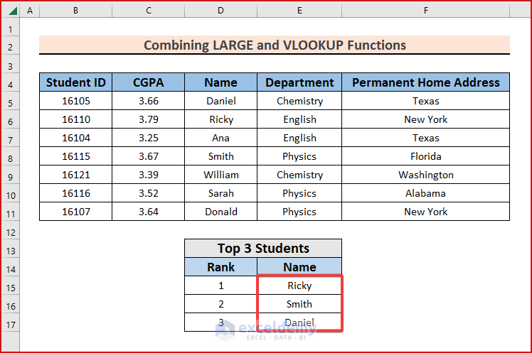
The dataset showcases students’ names, IDs, their CGPAs (Cumulative Grade Point Average), their departments, and their home addresses. To see the names of the top 3 students with the highest CGPAs.
Steps:
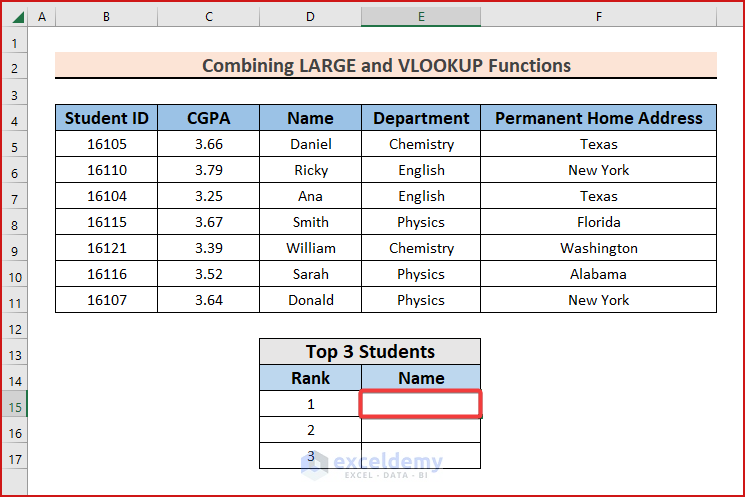
- Select a cell where to display the highest CGPA. Here, E15.
- Enter the formula into the cell.
=VLOOKUP(LARGE($C$5:$C$11,D15),$C$5:$F$11,2,0)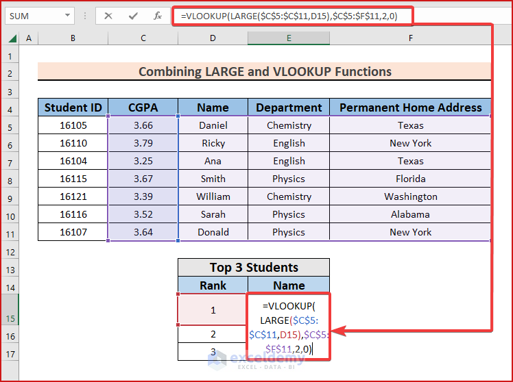
Formula Breakdown
- LARGE($C$5:$C$11,D15) —> finds the n-th largest value (n=D15) in C5:C11. Here, D15=1, looks for the highest CGPA value.
- VLOOKUP(LARGE($C$5:$C$11,D15),$C$5:$F$11,2,0)—> The VLOOKUP function finds the highest CGPA value in C5:C11. It returns the exact match of the text data corresponding to the highest CGPA value in the 2nd column (Name) of the selected range (C5:F11).
- Press Enter to see the result.
Ricky has the highest CGPA (3.79). His name is displayed in E15.

- Drag down the Fill Handle to autofill the formula in E16:E17.
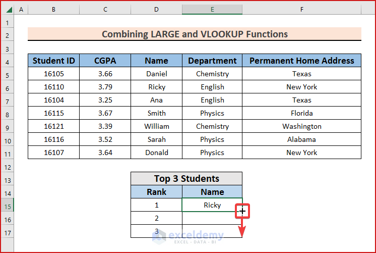
The top 3 students’ names are displayed.
Read More: How to Use Excel Large Function with Text
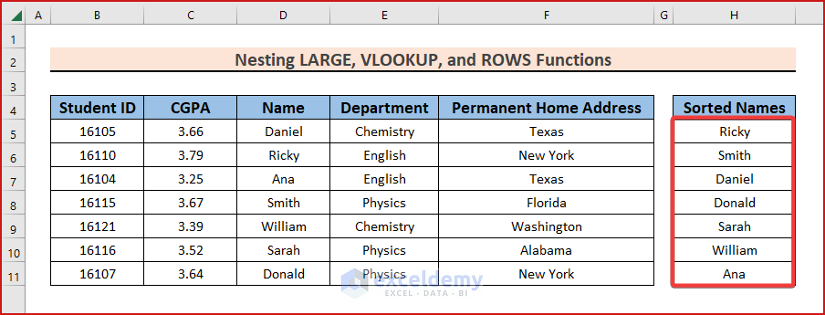
Method 2 – Nest the LARGE, VLOOKUP, and ROWS Functions to Sort Text data in Descending Order in Excel
Steps:
- Select a cell to sort the names. Here, H5.

- Enter the formula into the cell.
=VLOOKUP(LARGE($C$5:$C$11,ROWS(C$5:$C5)),$C$5:$F$11,2,0)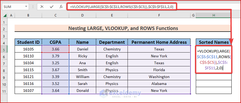
Formula Breakdown
- ROWS(C$5:$C5)—> Returns the row number of the reference.
- LARGE($C$5:$C$11,ROWS(C$5:$C5))—> The LARGE function finds the largest number in C5:C11, in descending order.
- VLOOKUP(LARGE($C$5:$C$11,ROWS(C$5:$C5)),$C$5:$F$11,2,0)—> The VLOOUP function returns the exact match, corresponding to the CGPA value in column 2 (Name) of the selected range (C5:F11).
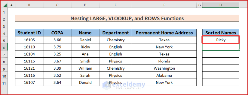
- Press Enter to see the result.
- Drag down the Fill Handle to see the result in the rest of the cells.
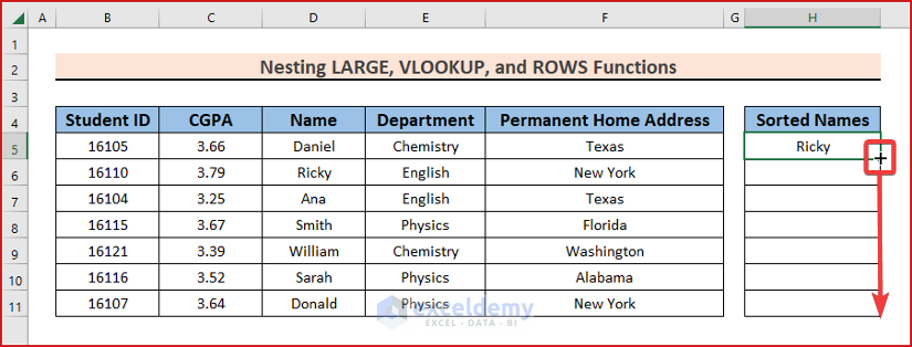
This is the output.
Notes
The LARGE and the VLOOKUP functions have limitations:
- The VLOOKUP function returns data from columns that are situated on the right-hand side of the lookup value only.
- The LARGE function will not work if the second argument of the function (n-th value) is either a negative number or the assigned value is greater than the number of rows in the specified range.
- The LARGE function will not work if the selected array is empty or does not include numeric values.
Read More: How to Use Excel LARGE Function with Criteria
Download Practice Book
Download the practice workbook.
Related Articles
- How to Use Excel Large Function in Multiple Ranges
- How to Use Excel LARGE Function with Duplicates in Excel
- How to Lookup Next Largest Value in Excel
- How to Use VBA Large Function in Excel
- How to Find Second Largest Value with Criteria in Excel
- How to Use LARGE and SMALL Function in Excel
<< Go Back to Excel LARGE Function | Excel Functions | Learn Excel


Thank you for explaining how to use the LARGE function with the VLOOKUP function in Excel. I find this information very helpful in my work. However, I am curious if there are any limitations to using these functions together? Can they be used with larger datasets or is there a point where they become inefficient? Thank you for your article and any additional information you can provide.
Hi YOGAAGA
Thank you very much for your comment. A few limitations while working with these functions have been discussed in the NOTES section. Please go through them. In addition, here in the dataset, the VLOOKUP function has been used in combination with the LARGE function. Both the VLOOPUP and LARGE functions go through the entire range of data every time they are called. The LARGE function needs to sort the data before determining the result. The VLOOKUP function looks for the data in a specified range. The whole process can be computationally expensive in large datasets. So, this formula can be time-consuming when dealing with large amounts of data.
Moreover, this formula may return identical values if it encounters duplicates in the dataset. For example, in our dataset, if there are multiple students with the same CGPA, the formula will return the same student’s name for each duplicate value.
Thank you once again. Let me know in the comments if you have any further queries.
Regards,
Md. Abu Sina Ibne Albaruni
Team ExcelDemy