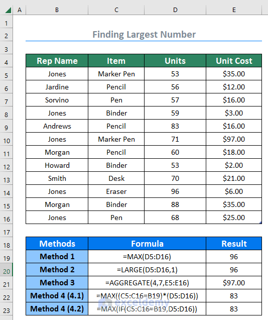
We’ll use a large dataset and determine the largest number from it. The image shows the overview of the functions we’ll use.
How to Find the Largest Number in Excel: 2 Ways
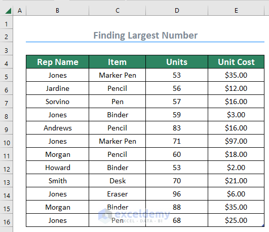
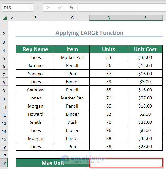
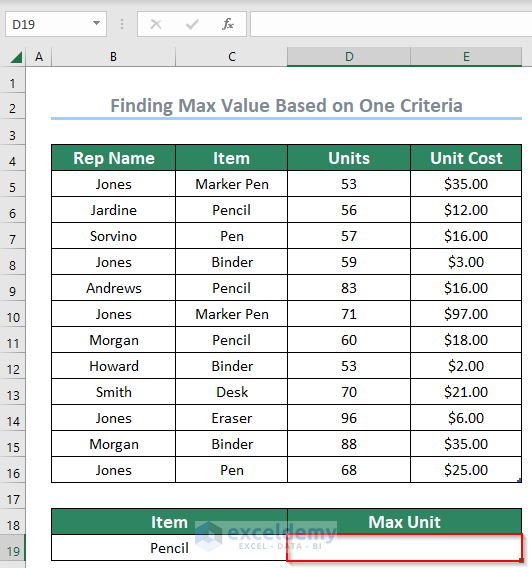
We have a concise dataset that contains 13 rows and 4 columns of Rep Name, Item, Units, and Unit Cost.
Method 1 – Use Excel Functions to Find the Largest Number Within a Range in Excel
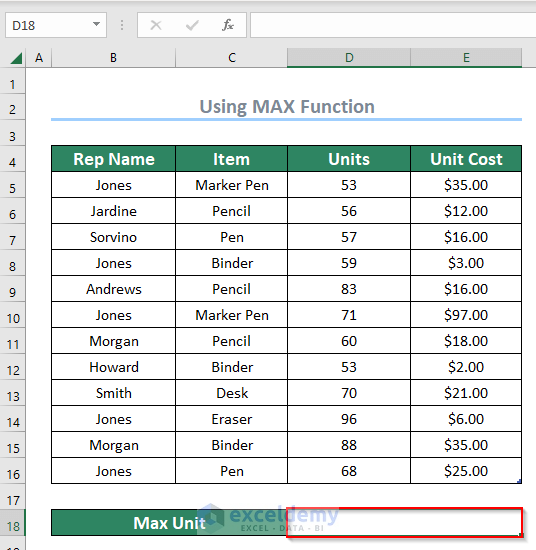
Case 1 – Using the MAX Function
We’ll find the largest value in the Units column.
Steps:
- Select your preferred cell (i.e. D18) to have your output.
- Insert the following formula:
=MAX(D5:D16)D5:D16 is the range of values of the Units column.
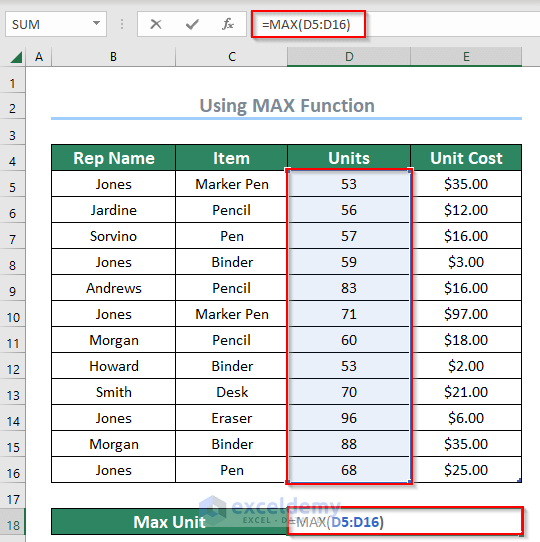
- Press the Enter key and the result will be shown in cell D18.
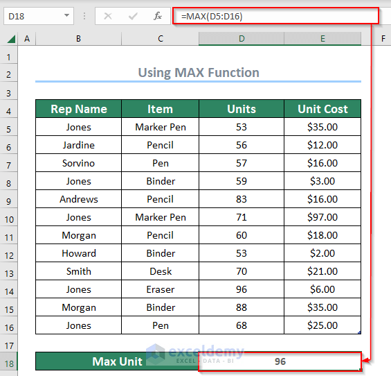
We got the Max Unit that contains the largest value of the specified range.
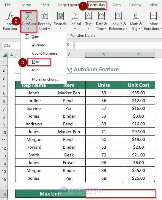
Another way of finding the largest value in a dataset is using the AutoSum feature.
Alternative steps:
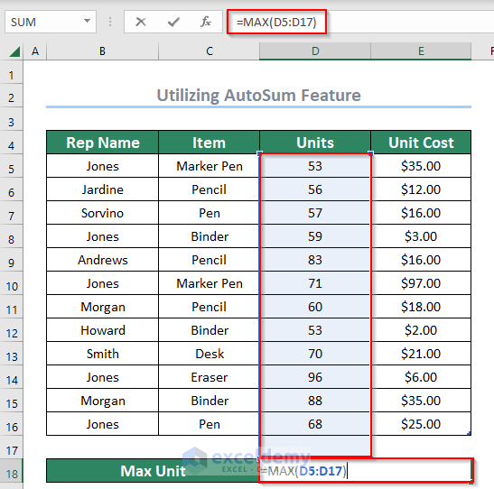
- Select the range you want to check (D5:D17).

- Select the Formulas tab.
- Click AutoSum.
- Select Max from the drop-down.
- This inserts a formula.
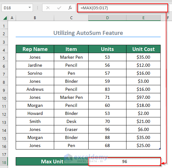
=MAX(D5:D17)D5:D17 is the range of values of the Units column.
- Press the Enter key and you will get your result in cell D18.
Case 2 – Applying the LARGE Function
Steps:
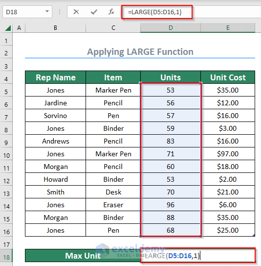
- Select cell D18 to show the output.
- Insert the following formula in cell D18 to find the largest value.
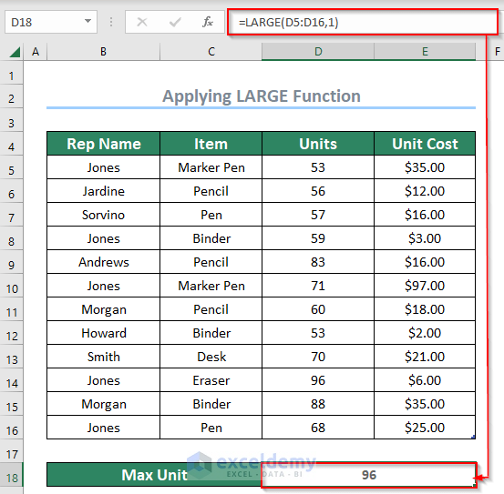
=LARGE(D5:D16,1)D5:D16 is the array or range of values of the Units column and 1 is the k value which represents the position of data you want to get. So, 1 means the first largest value.
- Press the Enter key. You will get your result in cell D18.
Read More: How to Use Excel Large Function in Multiple Ranges
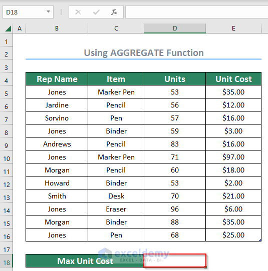
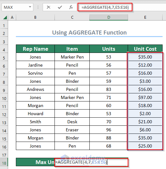
Case 3 – Using the AGGREGATE Function
We want to know the Max Unit Cost of the Unit Cost column.
Steps:
- Select cell D18 to show output.
- Insert the following formula:
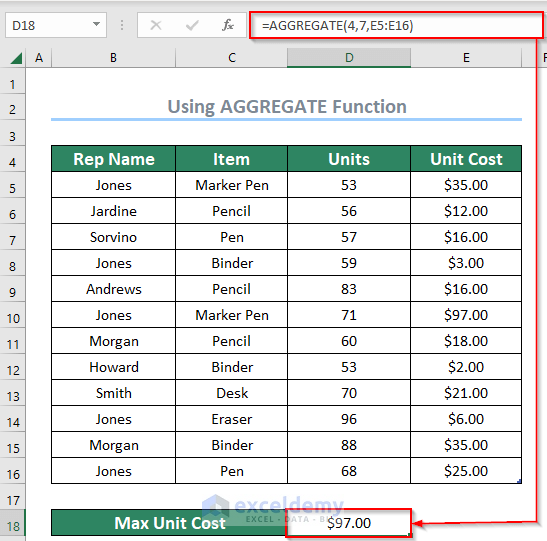
=AGGREGATE(4,7,E5:E16)Here, 4 indicates that we want to apply the MAX function to get the highest value, 7 indicates that we are ignoring hidden rows and error values, and E5:E16 is the array range of the Unit Cost column.
- Press the Enter key. The output will be shown in cell D18.
Method 2 – Finding the Largest Number Within a Range Based on Criteria
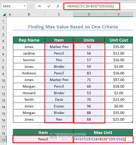
Case 1 – Calculating the Maximum Value by Using the MAX Function
In this dataset, the Pencil was sold in different units, and we want to get the highest such value.
Steps:
- Select cell B19 to enter the criterion which is Pencil.
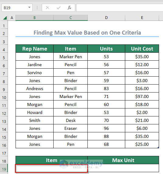
- Enter the criterion.
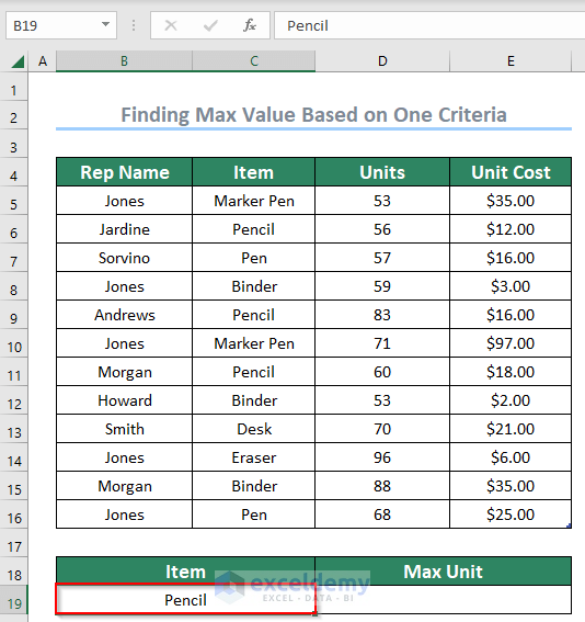
- Select cell D19 to show output.
- Insert the following formula in cell D19 to find the largest value.
=MAX((C5:C16=B19)*(D5:D16))C5:C16 is the range of the Item column, D5:D16 is the range of the Units column, and B19 is the criterion.
Formula Breakdown
- B19 → Pencil is the criterion located in cell B19.
- MAX((C5:C16=‘Pencil’)*(D5:D16)) → becomes
- MAX(({“Marker Pen”;“Pencil”;“Pen”;“Blinder”;“Pencil”;“Marker Pen”;“Pencil”;“Blinder”;“Desk”;“Eraser”;“Blinder”;“Pen”}=“Pencil”)*(D5:D16)) → returns TRUE for the exact match Pencil and otherwise returns FALSE.
- Output → MAX(({FALSE;TRUE;FALSE;FALSE;TRUE;FALSE;TRUE;FALSE;FALSE;FALSE;FALSE;FALSE})*(D5:D16))
- MAX(({“Marker Pen”;“Pencil”;“Pen”;“Blinder”;“Pencil”;“Marker Pen”;“Pencil”;“Blinder”;“Desk”;“Eraser”;“Blinder”;“Pen”}=“Pencil”)*(D5:D16)) → returns TRUE for the exact match Pencil and otherwise returns FALSE.
- MAX({FALSE;TRUE;FALSE;FALSE;TRUE;FALSE;TRUE;FALSE;FALSE;FALSE;FALSE;FALSE}*(D5:D16))
- MAX({FALSE;TRUE;FALSE;FALSE;TRUE;FALSE;TRUE;FALSE;FALSE;FALSE;FALSE;FALSE}*{53;56;57;59;83;71;60;53;70;96;88;68}) → returns 0 for FALSE.
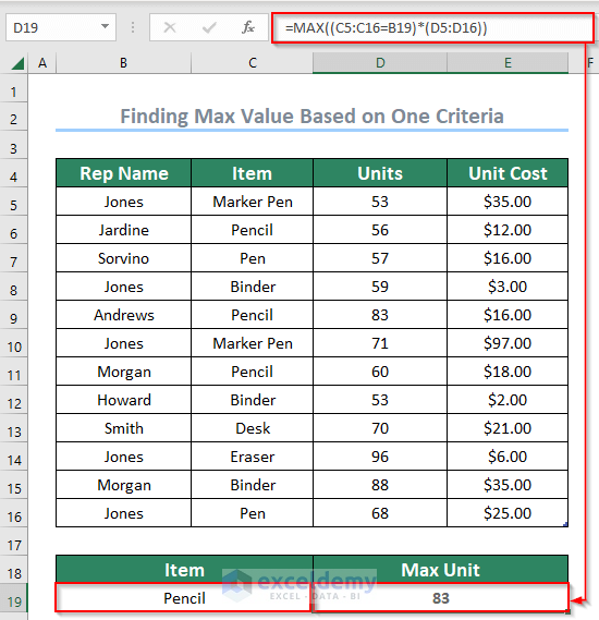
- Output → MAX({0;56;0;0;83;0;60;0;0;0;0;0})
- Output → 83
- Output → MAX({0;56;0;0;83;0;60;0;0;0;0;0})
- Press the Enter key. The output will be shown in cell D19.
Case 2 – Using a Combination of MAX and IF Functions
Steps:
- Select cell B19 to enter the criteria which is Pencil.
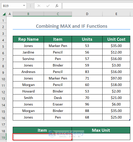
- Enter the criterion.
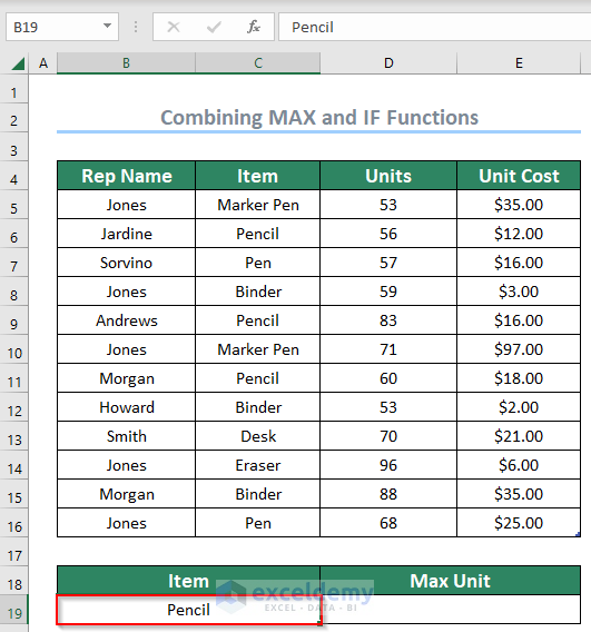
- Select cell D19 to get output.
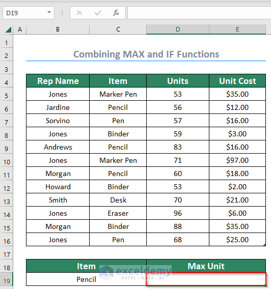
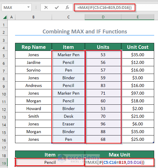
- Insert the following formula:
=MAX(IF(C5:C16=B19,D5:D16)))C5:C16 is the range of the Item column, D5:D16 is the range of the Units column, and B19 is the criterion.
Formula Breakdown
- B19 → Pencil is the criterion located in cell B19.
- MAX(IF(C5:C16=B19,D5:D16)) → becomes
- MAX(IF({“Marker Pen”;“Pencil”;“Pen”;“Blinder”;“Pencil”;“Marker Pen”;“Pencil”;“Blinder”;“Desk”;“Eraser”;“Blinder”;“Pen”}=“Pencil”,D5:D16)) → returns TRUE for the exact match Pencil and otherwise returns FALSE.
- MAX(IF({FALSE; TRUE; FALSE; FALSE; TRUE; FALSE; TRUE; FALSE; FALSE; FALSE; FALSE; FALSE}, D5:D16)) → The IF function will give us the numeric value for TRUE.
- Output → MAX({FALSE;56;FALSE;FALSE;83;FALSE;60;FALSE;FALSE;FALSE;FALSE;FALSE})
- MAX({0;56;0;0;83;0;60;0;0;0;0;0})
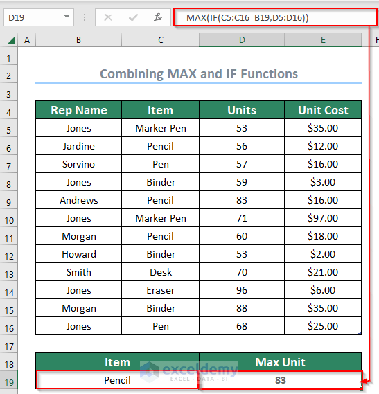
- Output → 83
- Press the Enter key. The output will be shown in cell D19.
Read More: How to Use Excel LARGE Function with Criteria
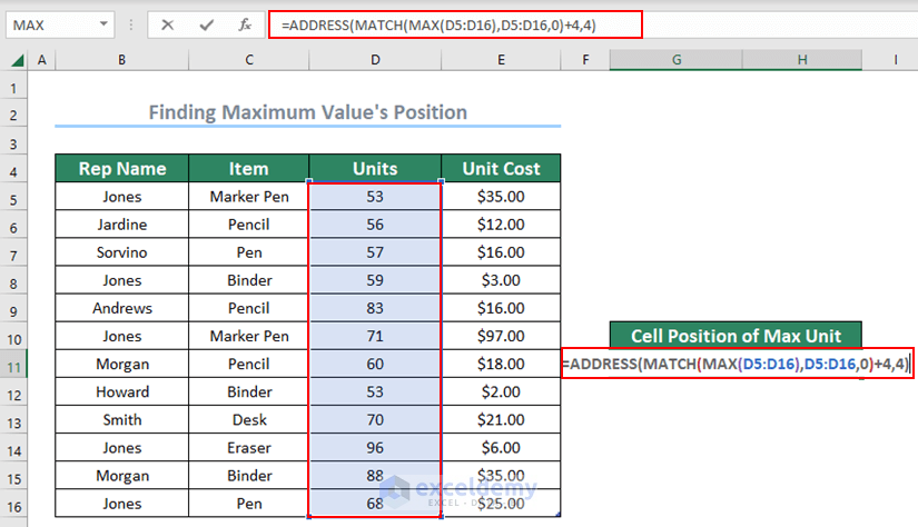
How to Find the Position of the Largest Number in Excel
Steps:
- Insert the following formula in cell G11 to find the cell address of the maximum value, then press the Enter key.
=ADDRESS(MATCH(MAX(D5:D16),D5:D16,0),+4,4)D5:D16 is the array or range of values of the Units column and 4 indicates that there are four extra rows before starting the values.
Formula Breakdown
- MAX(D5:D16) → returns the maximum value of the range D5:D16.
- ADDRESS(MATCH(MAX(D5:D16),D5:D16,0)+4,4) → becomes
- Output → ADDRESS(MATCH(96,D5:D16,0)+4,4)
- MATCH(96, D5:D16,0) → The MATCH function returns the maximum exact match value (96) from range D5:D16. 0 is set to return the exact match.
- MATCH(96,D5:D16,0) → becomes
- Output → ADDRESS(10+4,4)
- MATCH(96,D5:D16,0) → becomes
- ADDRESS(10+4,4) → The ADDRESS function creates a cell reference based on a given column and row number.
- ADDRESS(10+4,4) → becomes
- Output → ADDRESS(14,4)
- Output → $D$14
- Output → ADDRESS(14,4)
- ADDRESS(10+4,4) → becomes
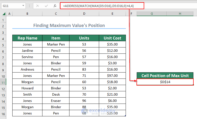
We got the maximum value of the Units column which is 96, and its cell address which is $D$14 by applying MAX, MATCH, and ADDRESS functions.
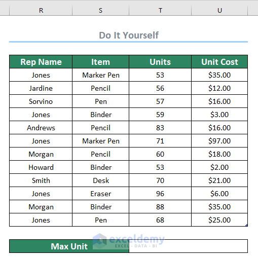
Practice Section
We’re providing the practice dataset so you can test these methods.
Download the Practice Workbook
Related Articles
- How to Lookup Next Largest Value in Excel
- How to Use Excel LARGE Function with Duplicates in Excel
- How to Use LARGE Function with VLOOKUP Function in Excel
- How to Find Second Largest Value with Criteria In Excel
- How to Use Excel LARGE Function with Text
- How to Use LARGE and SMALL Function in Excel
<< Go Back to Excel LARGE Function | Excel Functions | Learn Excel

