INDEX, MATCH and MAX with Multiple Criteria in Excel

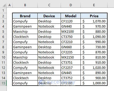
Combining INDEX, MATCH, and MAX functions is one of the most comprehensive formulas which will let you extract maximum or largest values under multiple criteria. The screenshot represents our dataset that will be used in this article to show the applications of numerous functions. The table shows 4 columns with the names of computer brands, device types, their model names, and prices.

Introduction to INDEX, MATCH, and MAX Functions

1. INDEX

• Formula Syntax:

=INDEX(array, row_num, [column_num])

or,

=INDEX(reference, row_num, [column_num], [area_num])

• Activity:

Returns a value of reference of the cell at the intersection of the particular row and column, in a given range.

• Example:

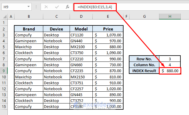
Based on our dataset mentioned earlier, we’ll use the INDEX function to find the value of the cell at the intersection of the 3rd row and 4th column from the array of B3:E15. So, our formula in Cell H9 will be:

After pressing Enter, you’ll get the return value as $880.00 which lies at the intersection of the 3rd row and 4th column in the selected array.

2. MATCH

• Formula Syntax:

=MATCH(lookup_value, lookup_array, [match_type])

• Activity:

Returns the relative position of an item in an array that matches a specified value in a specified order.

• Example:

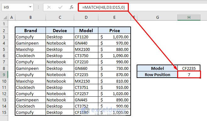
By inserting the MATCH function for our dataset, we’ll find out which row contains model CF2235. So, the related formula in Cell H9 will be:

Now press Enter and you’ll be shown ‘7’ as the result. It means the selected model name is lying at the 7th row in the column of Model (Column D).

3. MAX

• Formula Syntax:

=MAX(number1, [number2],…)

• Activity:

Returns the largest value in a set of values, ignores logical values and text strings.

• Example:

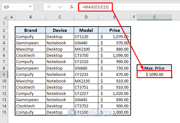
We’ll use the MAX function to find the maximum or highest price from Column E. So we have to type in Cell G9:

After pressing Enter, you’ll be shown the highest or maximum price instantly from the column with the Price header.

INDEX, MATCH and MAX with Multiple Criteria in Excel: 2 Suitable Ways

Method 1 – Using INDEX, MATCH and MAX Functions Together to Get the Maximum Price

Steps:

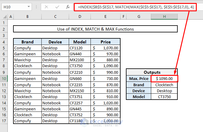
• Select the output Cell H10 and insert the following:

• Press Enter and you’ll get the highest price and can use it as the basis for the item’s information.

How Does This Formula Work?

➤ MAX function here pulls out the largest or maximum value from the range of Cells E5:E17.

➤ MATCH function finds out the row position of that maximum value.

➤ Within the INDEX function, B5:E17 is the entire array where our data extraction functions are being applied and the other arguments are showing row number and column number.

➤ Here, ‘4’ has been chosen as a column number since the price list is present in the 4th column of the selected array.

➤ INDEX function now extracts the data from Column E based on the row and column criteria.

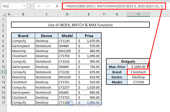
• Now, we’ll find out the brand name for the highest price. So in our output Cell H11, the related formula will be:

Here, 1 is the column number for the INDEX function as all brand names are present in the 1st column of the selected array.

• In Cell H12, we’ll determine the type of device for the maximum price. The column number will be 2. So, the embedded formula will be in Cell H12:

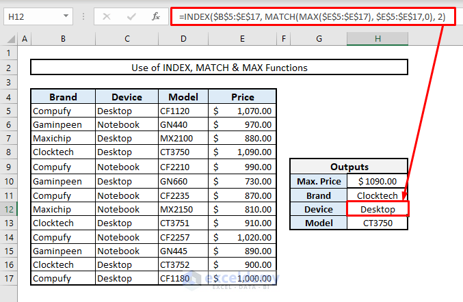
• Finally, we’ll determine which model has the maximum price. So, in Cell H13, the formula will be:

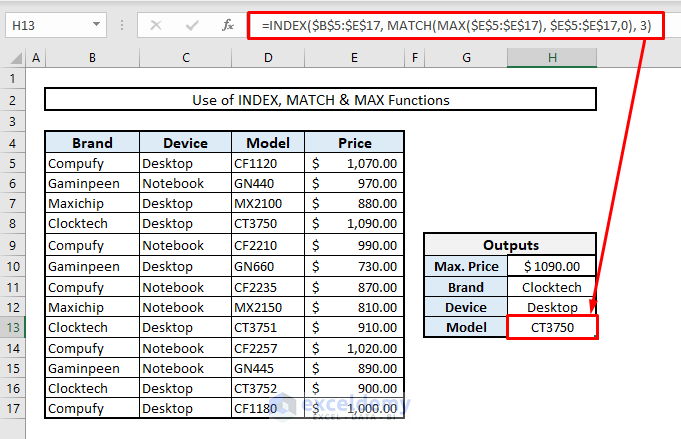
Method 2 – Using INDEX, MATCH, and MAX Functions Together to Find the Latest Date

In our modified dataset below, the Date of Manufacture column has been added to assign dates. We’ll find out the latest date among all.

Steps:

• Select Cell H10 and input:

• Press Enter.

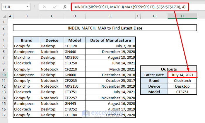
As the dates are present in the 4th column of the selected array, we’ve assigned the column number of the INDEX function as 4. If we want to extract the model name, device type, and brand name for that particular date of manufacture, we have to simply change the column number for the INDEX function based on the criteria position in the array.

Alternative Methods to INDEX, MATCH, and MAX Functions

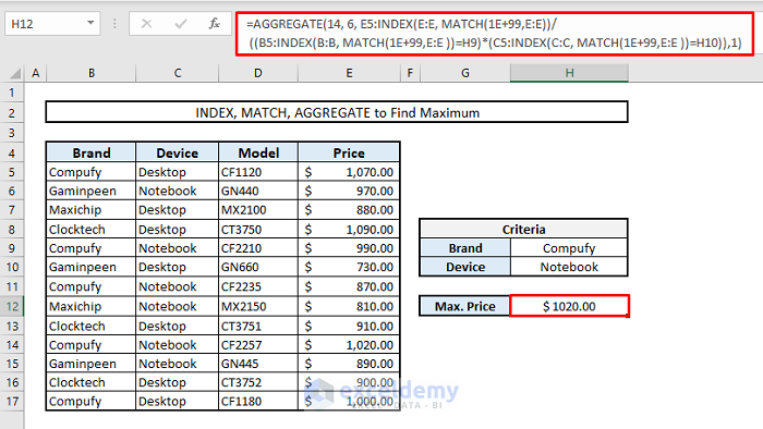
Method 3 – Combining INDEX, MATCH, and AGGREGATE Functions to Determine Maximum Value with Multiple Criteria

Let’s learn more about the AGGREGATE function first before applying the function in this section.

• Formula Syntax:

=AGGREGATE(function_num, options, array, [k])

or,

=AGGREGATE(function_num, options, ref1, ref2, [ref3],…)

• Arguments:

function_num- A list of 19 functions with serial numbers will appear. You have to select the function required with the serial number.

options- An option to choose that will ignore the error or numerical data.

array- Selected array or range of cells where the formula will work

[k]- serial number or position in the array based on the return values

• Activity:

Returns an aggregate in a list or database.

We’re going to determine the highest price of the notebook of the Compufy brand.

Steps:

• Select the output Cell H12 and insert:

• Press Enter.

How Does This Formula Work?

➤ Inside the array, 14 is the Function Number that is assigned to the LARGE function.

➤ 6 has been chosen as Option Number which ignores the Error Values.

➤ In the 3rd argument, a complex array has been established. The dividend or numerator part returns an array with all prices from the list and it looks like-

{1070;970;880;1090;990;730;870;810;910;1020;890;900;1000}

➤ The divisor or denominator has two parts and both work with logical functions. The 1st part looks for the brand name Compufy in Column B while the 2nd part looks for a notebook device in Column C. Then the converted (TRUE=1, FALSE=0) and numerical logic values are multiplied alongside these two parts. So, the resultant array returns as-

{0;0;0;0;1;0;1;0;0;1;0;0;0}

➤ Now, all the prices found from the dividend will be divided with these logical values found from the divisor and it’ll return as-

{#DIV/0!;#DIV/0!;#DIV/0!;#DIV/0!;990;#DIV/0!;870;#DIV/0!;#DIV/0!;1020;#DIV/0!;#DIV/0!;#DIV/0!}

➤ Finally, the AGGREGATE function ignores all the Error Values and extracts the largest value from the array.

Method 4 – Fusing LARGE Function with INDEX-MATCH to Find the Highest or Largest Three

In our new and modified dataset below, prices of different models of 4 computer brands are present.

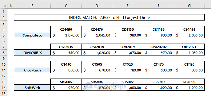
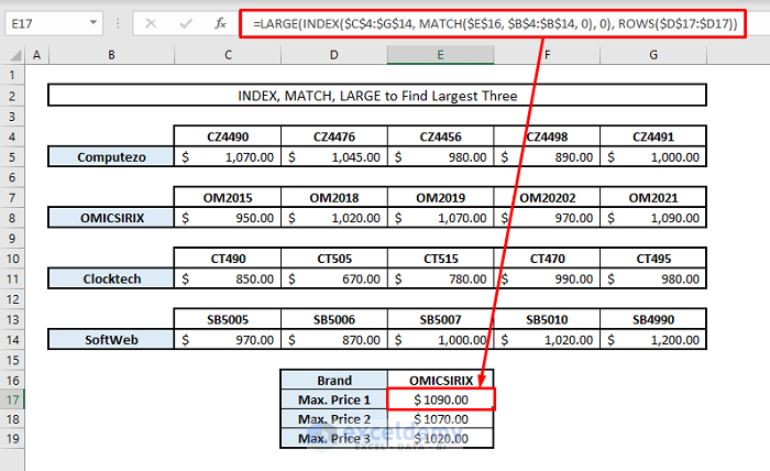
We’ll find out the highest three prices of a specific brand, let’s say OMICSIRIX.

Steps:

• In Cell E17, our formula for the mentioned criteria will be:

• Press Enter.
• To get the 2nd and 3rd highest prices, use the Fill Handle option to fill down the Cells E18 and E19.

Here, in Cell E16, if you change the brand name, you’ll find the highest 3 prices of that brand.

Method 5 – Incorporating MAX and IF Functions to Find the Maximum Value with Multiple Criteria

Based on our dataset, we’ll find out the maximum price of Compufy notebook with the combination of MAX and IF functions.

Steps:

• The formula in the output Cell H11 will be:

• Press Enter.

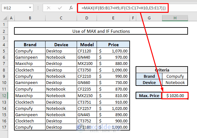
Inside this formula, IF functions are extracting the data based on the criteria. Then the MAX function will determine the largest one from them.

Method 6 – Using MAXIFS Function to Determine Maximum or Largest Value with Multiple Criteria

Let’s find out the maximum price of the Compufy notebook once again.

Steps:

• In Cell H12, our formula will be:

• Press Enter.

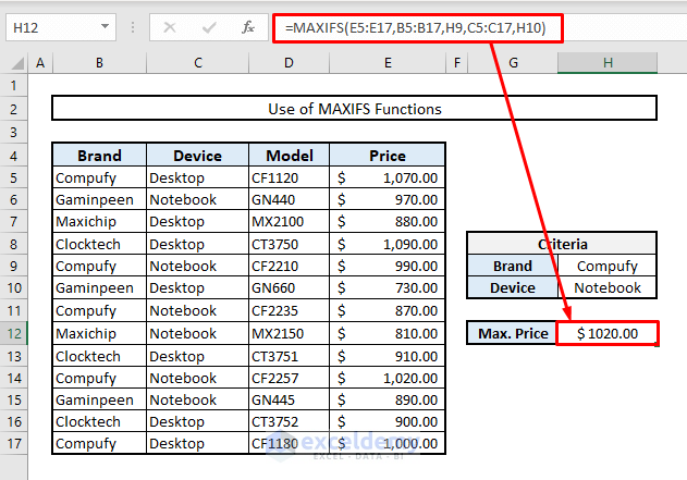
The MAXIFS function takes the range of data as 1st argument, 2nd argument here is the criteria range, and 3rd argument is the criteria, and finally returns the value from the 1st argument based on the inputted criteria. To add multiple criteria, we have to use Comma(,) between two criteria inside the function.

Download Practice Workbook

You can download our Excel Workbook that we’ve used to prepare this article. You’ll be able to modify input data and see how the table responds.

<< Go Back to Multiple Criteria | INDEX MATCH | Formula List | Learn Excel