How to Use INDEX MATCH with Multiple Criteria for Date Range

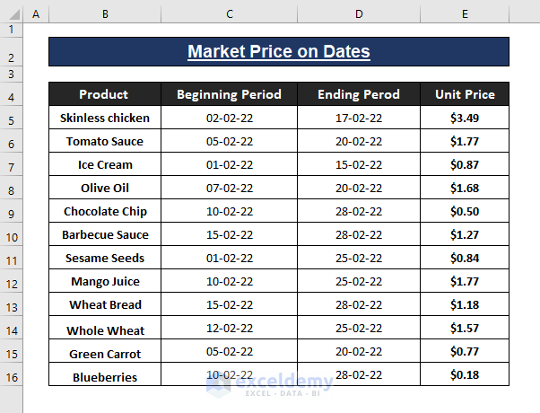
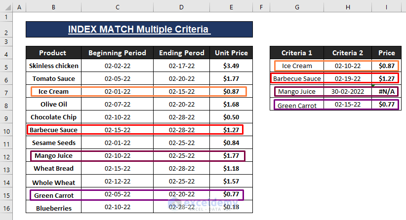
Let’s say we have certain products whose prices have remained stable for a certain period of time. We want to INDEX MATCH the prices for the given criteria.

How to Use INDEX MATCH with Multiple Criteria for Date Range: 3 Easy Ways

Method 1 – Using INDEX MATCH Functions for Multiple Criteria of Date Range

Suppose we want to see the price of an Ice Cream on 02-10-22 (month-day-year). If the given date falls between the offered period of time, we’ll have the price extracted in any blank cell.

Steps:

• Insert the following formula in the result cell (i.e., I5). As the formula in an array formula, Press Ctrl + Shift + Enter to apply it.

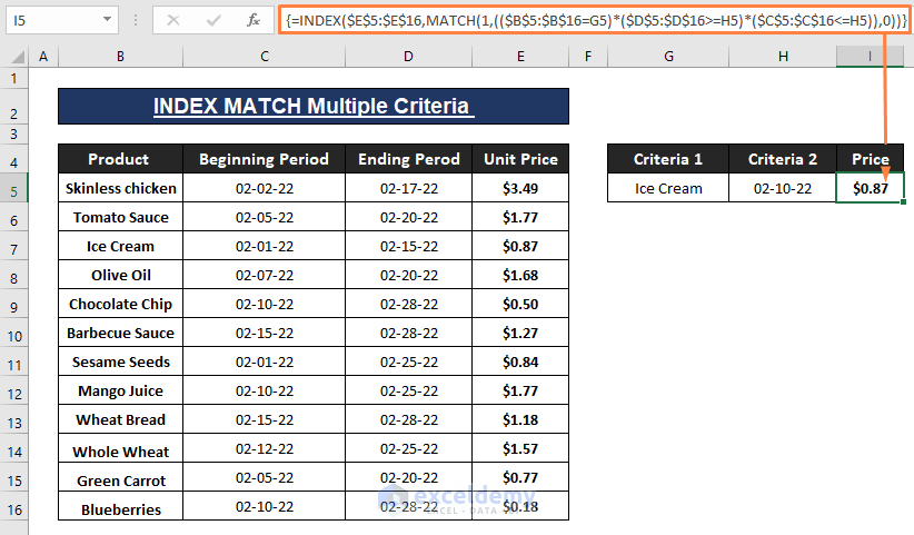
The formula returns the price of the Produce if the listed date falls in the given period of time (i.e., Date range) as depicted below.

Formula Breakdown:

Excel INDEX function finds a value of a given location within a given range. In our case, we use the MATCH function induced with the INDEX function. The MATCH function passes its result as a row number for entries that satisfy given criteria. The syntax of an INDEX function is

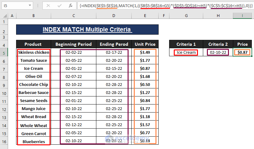
In the formula, $E$5$E$16 refers to the array argument. Inside the MATCH function $B$5:$B$16=G5, $D$5:$D$16>=H5, and  $C$5:$C$16<=H5 declare the criteria. To provide better identification, we color respective ranges in rectangles.

The MATCH function locates the position of a given value within a row, column, or table. As mentioned earlier, the MATCH portion passes the row number for the INDEX function. The syntax of the MATCH function is:

The MATCH portion is:

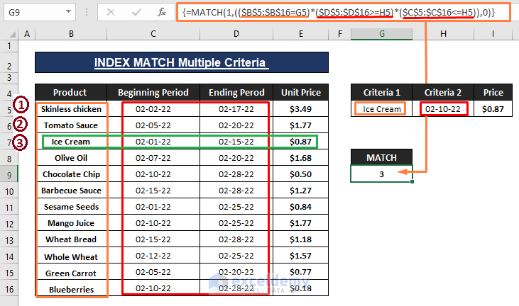
The MATCH portion assigns 1 as lookup_value, ($B$5:$B$16=G5)*($D$5:$D$16>=H5)*($C$5:$C$16<=H5) as lookup_array, and 0 declares the [match_type] as an exact match.

The used MATCH formula returns 3 as it finds Ice Cream in row number 3.

In case we have multiple products to extract their price from the dataset, you can drag the formula down to autofill the cells.

Method 2 – XLOOKUP Function to Deal with Multiple Criteria

The XLOOKUP function is only available in Excel 365. The syntax of the XLOOKUP function is:

Steps:

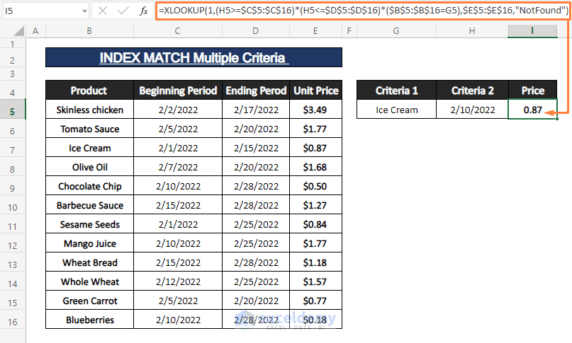
• Use the below formula in cell I5 and hit Enter.

The XLOOKUP formula returns the respective price of the product that satisfies the given criteria (i.e., Product and Date).

Formula Breakdown:

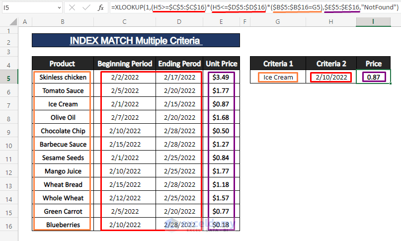
The XLOOKUP assigns 1 as its lookup argument, (H5>=$C$5:$C$16)*(H5<=$D$5:$D$16)*($B$5:$B$16=G5) as lookup_array, $E$5:$E$16 as return_array. Also, the formula displays Not Found text in case entries don’t fall in the date range. We indicated the assigned criteria in colored rectangles as depicted in the following image.

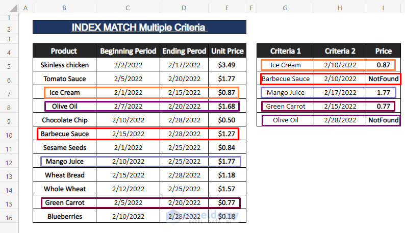
The formula displays Not Found if the given date criteria don’t expand within the given date range.

Method 3 – Use INDEX and AGGREGATE Functions to Extract a Volatile Price from Date Range

Some Products prices (i.e., crude oil, currency, etc.) are so volatile that they fluctuate each week or even day. We have the prices of a certain product in a week’s interval and want to find the price for the given dates.

Steps: Type the following formula in the result cell (i.e., E8) and hit Enter.

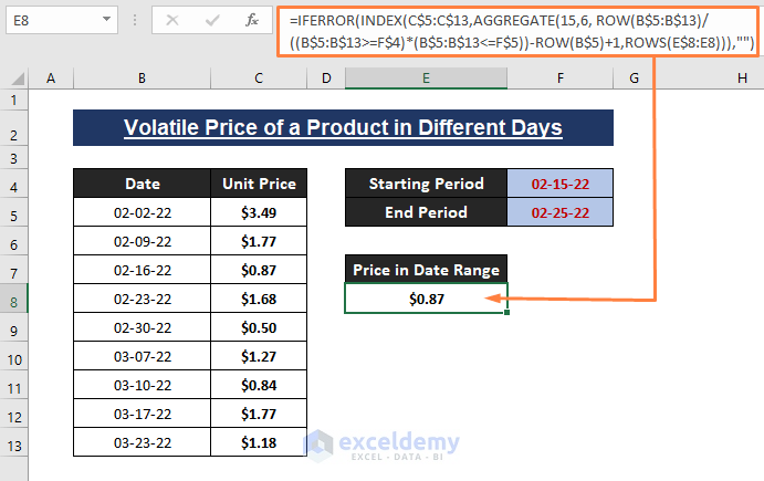
The 1^st price of the product dated 02-15-22 to 02-25-22 is $0.84. There may be more hits in the table depending on the date range, but this function will fetch the first recorded instance, if any exist.

Formula Breakdown:

The syntax of the AGGREGATE function is

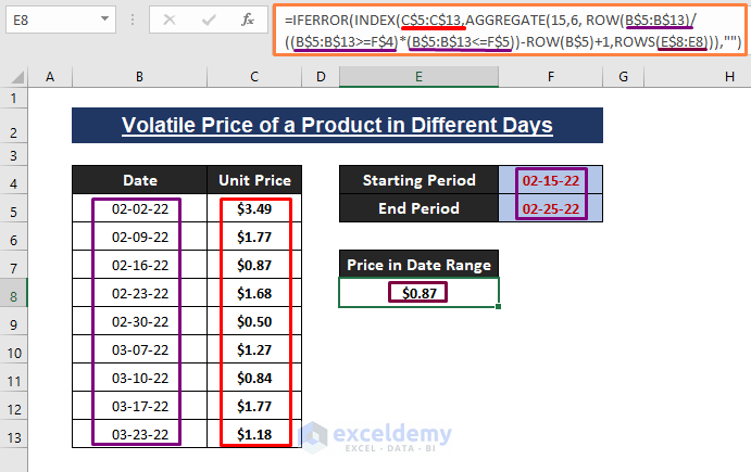
In the formula, =IFERROR(INDEX(C$5:C$13,AGGREGATE(15,6, ROW(B$5:B$13)/((B$5:B$13>=F$4)*(B$5:B$13<=F$5))-ROW(B$5)+1,ROWS(E$8:E8))),"");

AGGREGATE(15,6,ROW(B$5:B$13)/((B$5:B$13>=F$4)*(B$5:B$13<=F$5))-ROW(B$5)+1,ROWS(E$8:E8))) portion provides the row number to the INDEX function. C$5:C$13 is the array argument of the INDEX function.

Inside the AGGREGATE formula,

(B$5:B$13>=F$4)*(B$5:B$13<=F$5) returns 1 or 0 depending on whether the dataset dates fall in the range or not.

ROW(B$5:B$13)/((B$5:B$13>=F$4)*(B$5:B$13<=F$5)) returns an array of row numbers depending on the satisfying the date criteria. Otherwise, results in error values.

ROW(B$5:B$13)/((B$5:B$13>=F$4)*(B$5:B$13<=F$5))-ROW(B$5)+1 as ref1 results in an array of row numbers converted into index numbers otherwise in error values.

ROWS(E$8:E8) as ref2 results in row number and it’s an easy way to get row number as you apply the formula downward.

The number 15=function_num (i.e., SMALL), 6=options (i.e., ignore error values). You can choose function_num from 19 different functions and Options from 8 different options.

At last, AGGREGATE(15,6,ROW(B$5:B$13)/((B$5:B$13>=F$4)*(B$5:B$13<=F$5))-ROW(B$5)+1,ROWS(E$8:E8))) passes the n^th smallest index number of a row that satisfies the given criteria.

In case any error occurs, IFERROR(INDEX...),"") ignores all types of errors and transforms them into blanks.

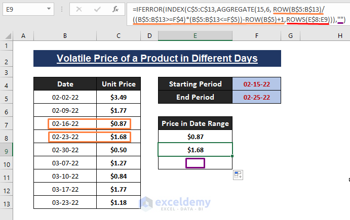
• Drag the Fill Handle to fetch other matched prices within the criteria date range. The IFERROR function results in blank cells if the formula encounters any errors.

Download Excel Workbook

<< Go Back to Multiple Criteria | INDEX MATCH | Formula List | Learn Excel