INDEX MATCH with 3 Criteria in Excel (4 Examples)

Method 1 – INDEX MATCH with 3 Criteria in Excel (Array Formula)

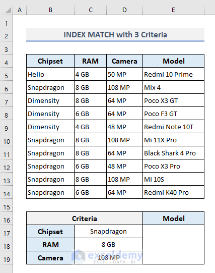
The following dataset contains a number of Xiaomi smartphone models with corresponding chipset models, RAM, and Camera specs. Based on the data available in the table, we’ll find a smartphone model that meets three different criteria from the first three specifications columns. For example, we want to find out a model that uses a Snapdragon chipset, has 8 GB RAM, and has a 108 MP camera, which are listed in a smaller table below.

• Select the output Cell E17 and type:

• Press CTRL + Shift + Enter to find the output as this is an Array formula. If you’re using Microsoft 365, then you have to press Enter only.

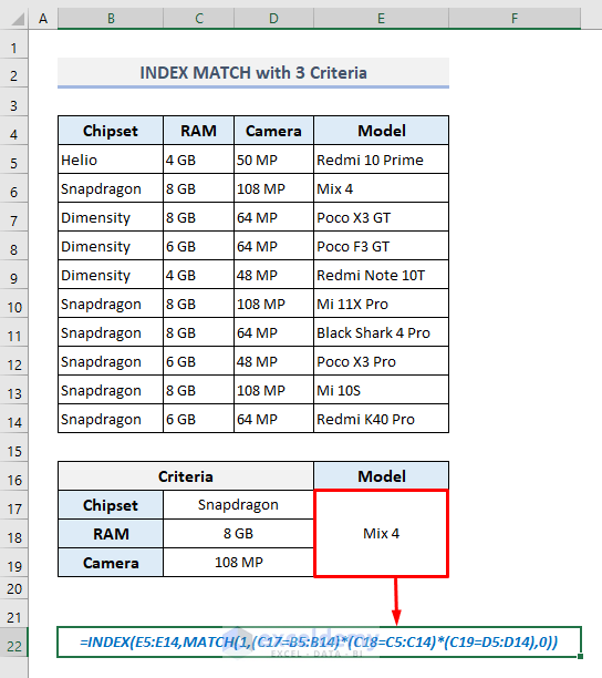
Here, the MATCH function extracts the row number based on the defined criteria. With its first argument as 1, the MATCH function looks for the value 1 in the lookup array (second argument) where all criteria have been met and it returns the corresponding row number. INDEX function then uses this row number to extract the smartphone model from Column E.

Method 2 – INDEX MATCH with 3 Criteria in Excel (Non-Array Formula)

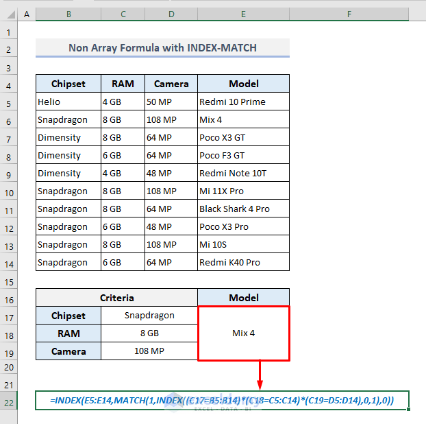
• Here’s another formula you can apply in the output Cell E17:

• After pressing Enter, you’ll get similar output as found in the previous section.

How Does the Formula Work?

• Inside the formula, the second argument of the MATCH function has been defined by another INDEX function which looks for multiple matched criteria and returns an array:

{0;1;0;0;0;1;0;0;1;0}

• MATCH function then looks for the value- 1 in this array and returns the corresponding row number of the first finding.
• Finally, the outer INDEX function extracts value from Column E based on the row number found in the preceding step.

Method 3 – Combination of IFERROR, INDEX, and MATCH Functions with 3 Criteria

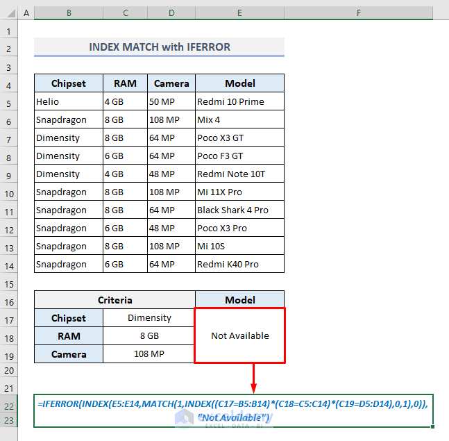
We can modify the formula to return a “Not Available” message if the given criteria are not matched.

The required formula in the output Cell E17 should be now:

After pressing Enter, we’ll see the defined message- “Not Available” as we have modified the criteria a bit that are unable to correlate with the data available in the table.

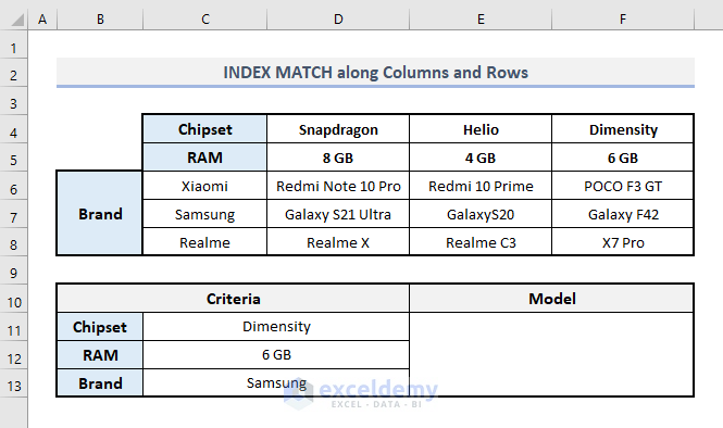
Method 4 – INDEX MATCH with 3 Criteria along Column(s) and Row(s) in Excel

In the final section, we’ll assign Chipset and RAM headers in two separate rows (4 and 5). We have also added two more smartphone brands in Column C. The range of cells from D6 to F8 represent the corresponding models based on the brands, chipsets, and RAMs across the column and row headers.

Based on this matrix lookup with multiple criteria along rows and columns, we’ll pull out the smartphone model in Cell E11 that meets the criteria defined in the range of cells D11:D13.

In the output Cell E11, the required formula under the specified conditions will be:

After pressing Enter, you’ll find the final output as shown in the screenshot below.

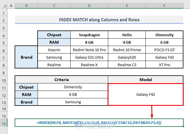
In this formula, the first MATCH function defines the row number from Column C that matches the given criteria for brands. In the third argument (column_num) of the INDEX function, the second MATCH function defines the column number by combining the chipset and RAM criteria.

Download Practice Workbook

You can download the Excel workbook that we have used to prepare this article.

<< Go Back to Multiple Criteria | INDEX MATCH | Formula List | Learn Excel