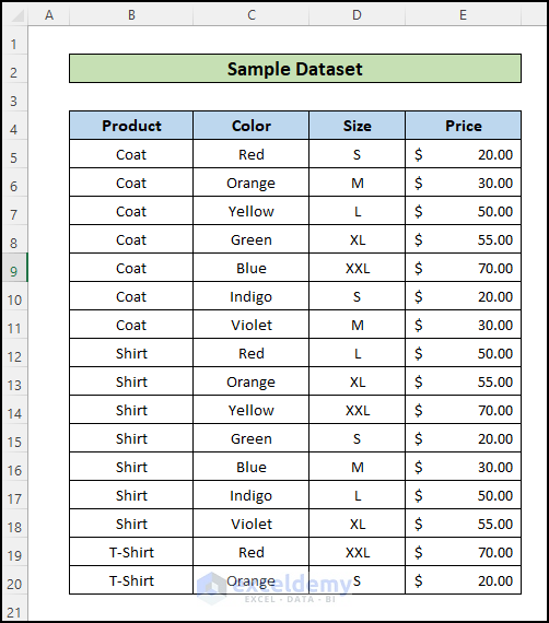
Dataset Overview
We’ll use a dataset that contains information about some clothing products. It has four columns, the name of the product, the Color, the Size, and the Price as you can see in the below image.
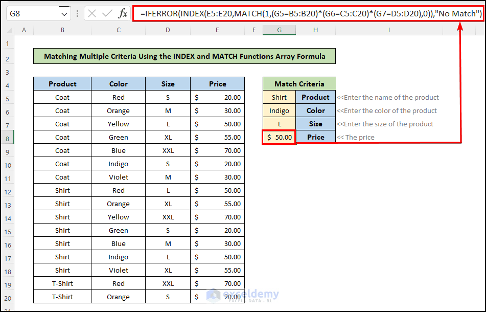
Method 1 – Using Array Formula with INDEX and MATCH Functions
Scenario: Fetch the Price of the Product (Cell B11) based on the product’s Name, Color, and Size.
Steps
- Insert the product name, color, and size in cells G5, G6, and G7.
- Then, enter the following formula in cell G8 to get the price for the product meeting those criteria:
=IFERROR(INDEX(E5:E20,MATCH(1,(G5=B5:B20)*(G6=C5:C20)*(G7=D5:D20),0)),"No Match")
Formula Breakdown
✅ The Multiplication Operation
→ (G5=B5:B20)*(G6=C5:C20)*(G7=D5:D20) = (Shirt = Product Column)*(Indigo = Color Column)*(L = Size Column) = {FALSE; FALSE;FALSE;FALSE;FALSE;FALSE;FALSE;TRUE;TRUE;TRUE;TRUE;TRUE;TRUE;TRUE;FALSE;FALSE}*(G6=C5:C20)*(G7=D5:D20)}
Checks each condition and returns TRUE/FALSE values.
→ {0;0;0;0;0;0;0;0;0;0;0;0;1;0;0;0}
The Multiplication Operator (*) converts these values to 0s and 1s and then performs the multiplication operation which converts all other values to 0s except the desired output.
✅ MATCH Function Operation:
→ MATCH(1,(0;0;0;0;0;0;0;0;0;0;0;0;1;0;0;0),0)) → 13
This function looks for the value 1 in the converted range and returns the position.
✅ INDEX Function Operation:
→ IFERROR(INDEX(E5:E20,13), “No Match”) → 50
This function returns the value in the 13th row of the price column which is the desired output. For cases where there are no matches, the INDEX function will return a #N/A error. For handling such errors and displaying a human-readable message, “No Match“, the IFERROR function is used.
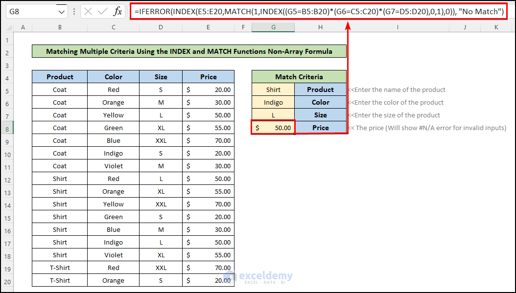
Method 2 – Using a Non-Array Formula of INDEX and MATCH Functions
Scenario: Fetch the Price of the Product (Cell B11) based on the product’s Name, Color, and Size.
Steps
- Insert the product name, color, and size in respective cells.
- Enter the following formula in cell G8 to get the price for the product that meets those criteria:
=IFERROR(INDEX(E5:E25,MATCH(1,INDEX((G5=B5:B25)*(G6=C5:C25)*(G7=D5:D25),0,1),0)),"No Match")
Formula Explanation
The new INDEX function converts the previous array formula to a non-array formula, making it easier for users unfamiliar with Excel’s array functions.
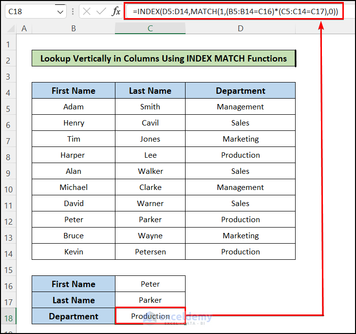
Method 3 – INDEX MATCH Formula for Multiple Criteria from Different Horizontal and Vertical Arrays in Excel
We will use a dataset containing the Names, Surnames and Departments of Salespeople.
Scenario: Fetch the Department of Peter Parker.
3.1 Lookup Vertically in Columns
Steps
- Click on cell C18 and insert the following formula:
=INDEX(D5:D14,MATCH(1,(B5:B14=C16)*(C5:C14=C17),0))
This gives you the desired result for your desired salesperson.
- Press Enter.
3.2 Lookup Horizontally in Rows
Steps
- Click on cell C10.
- Insert the following formula and press Enter:
=INDEX(C6:L6,MATCH(1,(C4:L4=C8)*(C5:L5=C9),0))
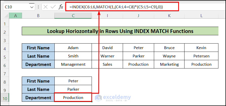
This provides the desired person’s department through the horizontal lookup.
Method 4 – INDEX MATCH Formula to Match Multiple Criteria from Arrays in Different Excel Sheets
Imagine you’re working on a business farm, and your boss assigns you a task: find the sales amount of different sales reps from another worksheet.
In this example, we have arbitrary data for ID, First Name, and Sale of workers. The goal is to find the Sale for a specific ID and a specific First Name in a different worksheet named Data.
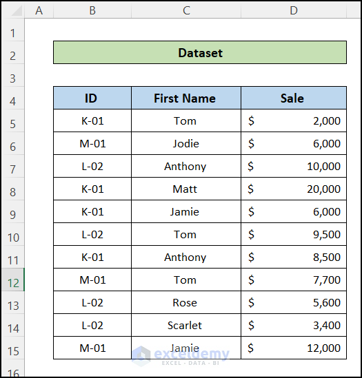
- Create another table in a new worksheet (let’s call it M01) with columns ID, First Name, and Sale.
- In cell D5 of the M01 worksheet, enter the following formula:
=INDEX(Data!$D$5:$D$15,MATCH(1,('M01'!B5=Data!$B$5:$B$15)*('M01'!C5=Data!$C$5:$C$15),0))
The formula searches for the specified ID and First Name in the Data worksheet and retrieves the corresponding Sale value.
- Apply the same formula to the rest of the cells in the M01 worksheet.
Method 5 – Using the COUNTIFS Function to Match Multiple Criteria from Different Arrays
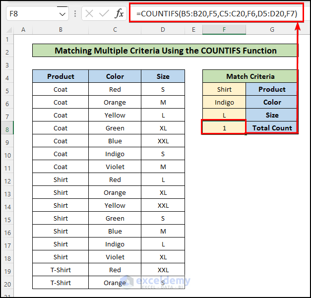
5.1 Using AND Logic for Multiple Criteria in Multiple Columns
AND logic requires all criteria to be matched. Let’s calculate the total number of rows based on the Name, Color, and Size criteria.
Steps
- Insert the product name, color, and size in cells F5, F6, and F7.
- Enter the following formula in cell F8 to count the cells that match the given criteria:
=COUNTIFS(B5:B20,F5,C5:C20,F6,D5:D20,F7)
Formula Breakdown
=COUNTIFS(B5:B20,F5,C5:C20,F6,D5:D20,F7) → COUNTIFS(Product Column, Shirt, Color Column, Indigo, Size Column, L) → 1
- The formula counts rows where all criteria (product name, color, and size) match.
- In this case, the result is 1 because there’s only one row that meets all criteria.
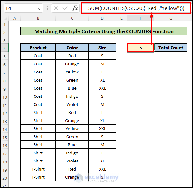
5.2 OR Logic for Multiple Criteria in the Same Column
OR logic means that if any criterion matches, the TRUE value is returned.
- To count the total number of rows where the color values are Red or Yellow, enter the following formula in cell F4:
=SUM(COUNTIFS(C5:C20,{"Red","Yellow"}))
Formula Breakdown
→ SUM(COUNTIFS(C11:C31,{“Red”,“Yellow”})) → SUM(COUNTIFS(Color column,{“Red”, ”Yellow”}))
- The COUNTIFS function checks each row for color values Red or Yellow and returns 3 for red and 2 for yellow.
- The SUM function adds these counts, resulting in a total of 5rows.
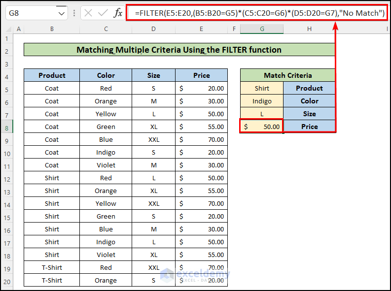
Method 6 – Using the FILTER Function
The FILTER function lives up to its name by allowing you to filter a range of cells based on specific criteria. Unlike other methods that involve multiple functions, here we rely solely on the FILTER function. Let’s break down the steps:
Steps
- Enter the name of the product, color, and size in the respective cells of the range F5:F7.
- Insert the following formula into cell F8 to retrieve the price of the product that meets all the specified criteria:
=FILTER(E5:E20,(B5:B20=G5)*(C5:C20=G6)*(D5:D20=G7),"No Match")
Formula Breakdown
Multiplication Operation:
The expression (B5:B20=G5)*(C5:C20=G6)*(D5:D20=G7) evaluates to a series of TRUE/FALSE values.
For example, if the product column equals “Shirt,” the color column equals “Indigo,” and the size column equals “L,” the result would be:
{FALSE; FALSE; FALSE; FALSE; FALSE; FALSE; FALSE; TRUE; TRUE; TRUE; TRUE; TRUE; TRUE; TRUE; FALSE; FALSE}
The Multiplication Operator (*) converts these values to 0s and 1s, effectively filtering out all other values except the desired output.
FILTER Function:
The FILTER function searches the Price column (E14:E34) using the index values from the previous step.
It returns the cell value where the corresponding index value is 1 (in this case, 50).
Note:
As of the time of writing this article, the FILTER function is only available in Excel 365. If you’re using other versions of Excel, be sure to explore alternative methods.
Download Practice Workbook
You can download the practice workbook from here:
<< Go Back to Multiple Criteria | INDEX MATCH | Formula List | Learn Excel
Get FREE Advanced Excel Exercises with Solutions!

him thanks for the wonderful tips! The formula keeps showing that there’s no match “1”.I’ve tried many different formula and it keeps showing the same warning. Could you please assist me? much appreciated!!
Hello Avery,
First of all, we would like to thank you for your appreciation. Again, thanks for taking the time to leave a comment about a problem that you’re facing. In our Excel file, the formula is working smoothly. You can follow the step-wise procedure thoroughly. If the problem in your file remains the same, then send the file to us. It will be easier for us to pinpoint the problem. We, the Exceldemy team, are always ready to solve users’ issues.
Regards,
Fahim Shahriyar Dipto
Excel and VBA Content Developer