Let’s have a quick look to the methods we will be using here and the relevant output.
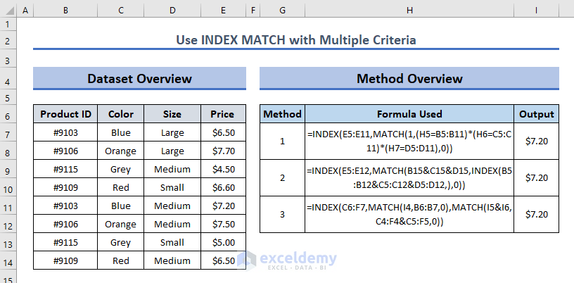
How to Use INDEX MATCH with Multiple Criteria in Excel: 3 Ways
The INDEX function returns a value or reference of the cell at the intersection of a particular row and column in a given range.
The MATCH function returns the relative position of an item in an array that matches a specified value in a specified order.
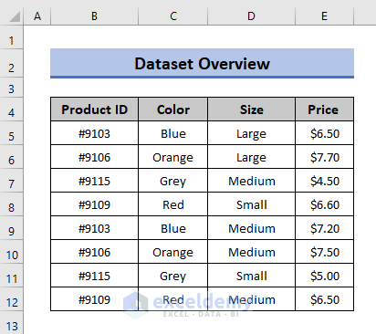
We will use the following dataset to explain 3 formulas. The dataset contains four columns with Product ID, Color, Size, and Price list of the products of a company.
Method 1 – Nested Formula Using INDEX and MATCH Functions
Let’s find out the price of a product from the dataset by matching the product ID, color, and size, which are provided in cells H5, H6, and H7.
- Use the following formula using Excel INDEX and MATCH function to get the result:
=INDEX(E5:E11,MATCH(1,(H5=B5:B11)*(H6=C5:C11)*(H7=D5:D11),0))
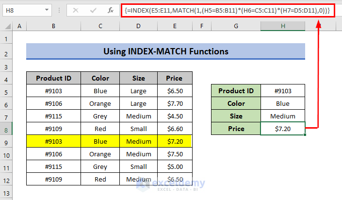
The formula matches criteria from the dataset and then shows a result (if one exists).
Formula Breakdown
- The MATCH function looks for the criteria Product ID, Color, and Size in ranges B5:B11, C5:C11, and D5:D11, respectively, from the dataset. The match type is 0, which gives an exact match.
- The INDEX function gets the price of that particular product from the range E5:E11.
Read More: INDEX-MATCH with Multiple Matches in Excel
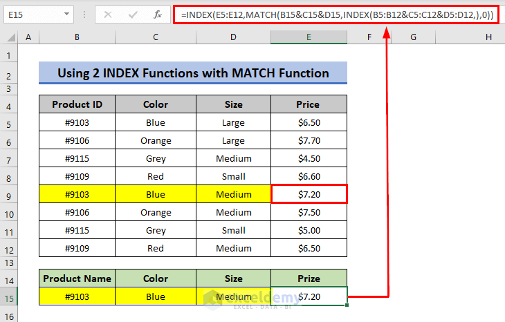
Method 2 – Nested Formula with Two INDEX Functions and MATCH Function
- Use the following formula:
=INDEX(E5:E12,MATCH(B15&C15&D15,INDEX(B5:B12&C5:C12&D5:D12,),0))
Formula Breakdown
- The MATCH function takes lookup values as B15, C15, and D15 using AND in between them. In the INDEX function are the lookup arrays for each of the lookup values: B5:B12, C5:C12, and D5:D12.
- The last argument of the MATCH function is 0 to give the exact match.
Read More: How to Use INDEX-MATCH Function for Multiple Results in Excel
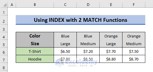
Method 3 – Using INDEX with Two MATCH Functions with Multiple Criteria
We have a modified version of the given dataset, including information about the Hoodie and T-shirt, arranged in the following way.
- Use this formula:
=INDEX(C6:F7,MATCH(I4,B6:B7,0),MATCH(I5&I6,C4:F4&C5:F5,0))
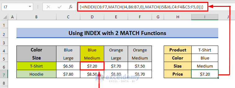
We have used two MATCH functions to match values from the dataset, one match for the row and the other for the column. Both MATCH formulas are nested inside an INDEX function.
Formula Breakdown
- The first MATCH formula matches the product name T-Shirt with the values in the column B (B6 and B7).
- The second MATCH formula takes two criteria, color and size (Blue and Medium) and compares them in the ranges C4:F4 and C5:F5, respectively.
- Both MATCH formulas are nested inside the INDEX formula as the second argument. The first argument of the INDEX formula takes the first argument as the range of data from which output will be extracted and the third is 0 for an exact match.
Read More: INDEX MATCH Formula with Multiple Criteria in Different Sheet
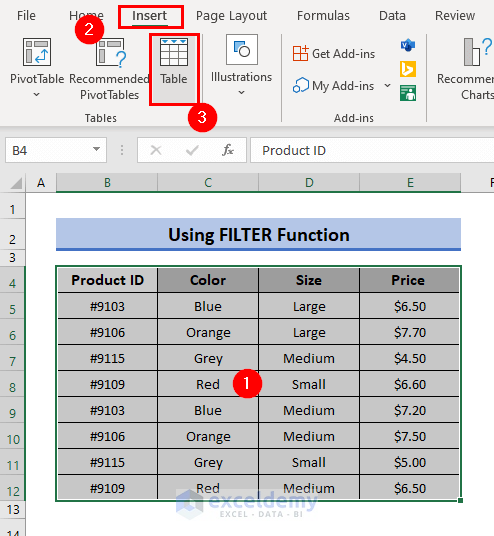
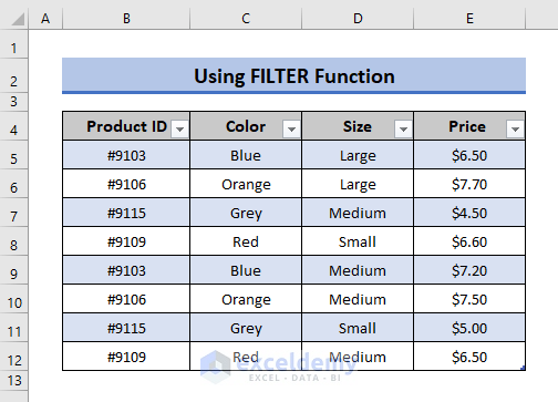
Alternative to the INDEX-MATCH: FILTER Function
If you are using Microsoft 365 which has dynamic arrays then you can use the FILTER function with multiple criteria as an alternative to the INDEX-MATCH formulas.
- Select the whole dataset.
- Choose Table from the Insert tab.
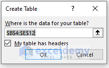
- Check the range of the table and tick My table has headers.
- Click OK.
- Your table will look like below.
- Suppose you have the 3 criteria (shown in the picture) using which you have to find the price of that particular product.
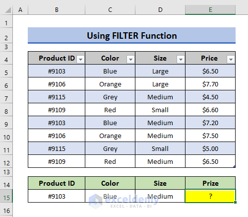
- Use the following formula in the cell where you want to see the result:
=FILTER(Table2[[Price ]],(Table2[Product ID]=B15)*(Table2[Color]=C15)*(Table2[Size]=D15))
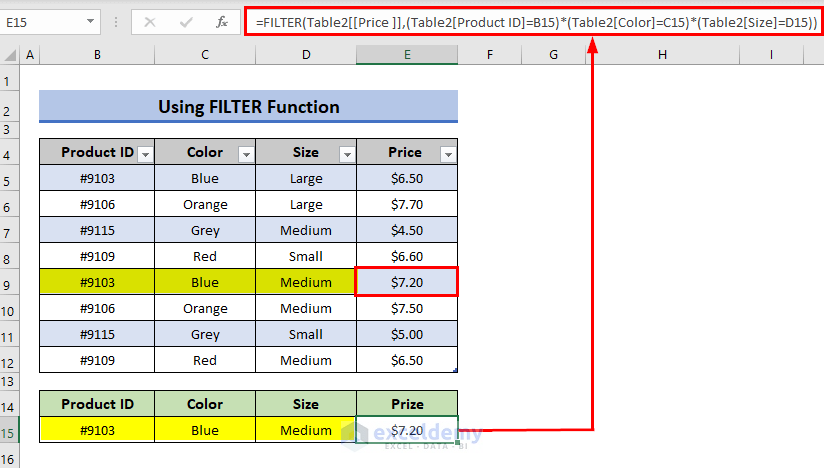
- The result will be shown in the cell.
Formula Breakdown
- The formula takes 3 arguments,
- The first argument is an array which is the range of data from which the return value will be extracted.
- The second argument is include which includes the criteria. In our case, the criteria are Product ID, Color, and Size.
- The third argument is empty_if which takes a return value if the result is empty. This one is optional and we do not require this in our case.
- It matches the criteria and provides the result from the range in the first argument.
Things to Remember
- Use Ctrl + Shift + Enter when applying array formulas. Newer Excel versions including Excel 365 also accept Enter.
- The FILTER function is only available for Microsoft 365 with a dynamic array feature.
Download the Practice Workbook
Download the practice workbook and practice yourself.
Use INDEX MATCH with Multiple Criteria in Excel: Knowledge Hub
<< Go Back to INDEX MATCH | Formula List | Learn Excel
Get FREE Advanced Excel Exercises with Solutions!

Thank you for these formula examples you provided in this article, Syeda. The INDEX MATCH INDEX example you showed really helped me figure out the formula I was looking for StackOverflow.
Thank you for your compliment, David!
Please click on the following link for more examples of the INDEX-MATCH combo:
https://www.exceldemy.com/tag/index-match-excel/