In this article, we will show you how to use the INDEX-MATCH formula in Excel to generate multiple results.
We’ll use the following dataset containing the Name and Marks columns to demonstrate our methods. We’ve used Microsoft 365 here, but you can use any available Excel version.
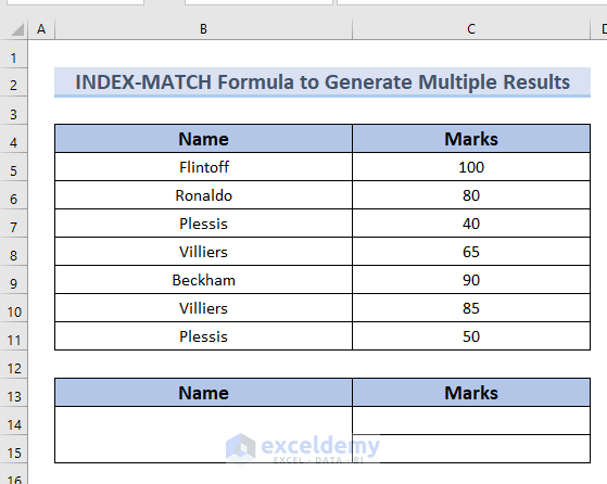
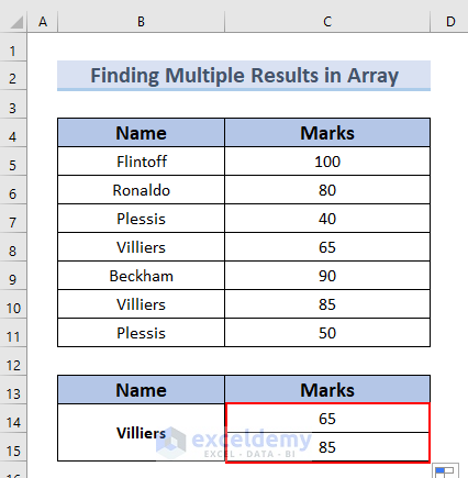
Example 1 – Finding Multiple Results in Arrays
In addition to an INDEX-MATCH formula, we’ll use the ISNUMBER, ROW, ROWS, and SMALL functions in our the formula.
Steps:
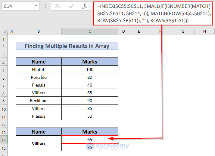
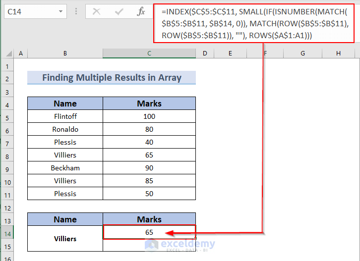
- Choose a name from the dataset (B5:B11) and put it in another cell to be used as a cell reference number later (e.g. Villiers in cell B14:B15).
- In another cell that you want as your result cell (e.g. cell C14), enter the following formula:
=INDEX($C$5:$C$11, SMALL(IF(ISNUMBER(MATCH($B$5:$B$11, $B$14, 0)), MATCH(ROW($B$5:$B$11), ROW($B$5:$B$11)), ""), ROWS($A$1:A1)))
Formula Breakdown
- MATCH($B$5:$B$11, $G$4, 0) → becomes,
- MATCH({“Flintoff”; “Ronaldo”; “Plessis”; “Villiers”; “Beckham”; “Villiers”; “Plessis”}, “Villiers”, 0)
- Output: {#N/A; #N/A; #N/A; 1; #N/A; 1; #N/A}
- MATCH({“Flintoff”; “Ronaldo”; “Plessis”; “Villiers”; “Beckham”; “Villiers”; “Plessis”}, “Villiers”, 0)
- Explanation: If the search value finds a match in the lookup array, then the MATCH function returns 1, otherwise it returns #N/A.
- ISNUMBER(MATCH($B$5:$B$11, $B$14, 0) → becomes,
- ISNUMBER({#N/A; #N/A; #N/A; 1; #N/A; 1; #N/A})
- Output: {FALSE; FALSE; FALSE; TRUE; FALSE; TRUE; FALSE}.
- ISNUMBER({#N/A; #N/A; #N/A; 1; #N/A; 1; #N/A})
- Explanation: As the IF function is unable to handle error values, the ISNUMBER function is being utilized here to convert the array values to Boolean values.
- IF(ISNUMBER(MATCH($B$5:$B$11, $B$14, 0)), MATCH(ROW($B$5:$B$11), ROW($B$5:$B$11)), “”) becomes,
- IF({FALSE; FALSE; FALSE; TRUE; FALSE; TRUE; FALSE}, MATCH(ROW($B$5:$B$11), ROW($B$5:$B$11)), “”) → becomes
- IF({FALSE; FALSE; FALSE; TRUE; FALSE; TRUE; FALSE}, {1; 2; 3; 4; 5; 6; 7}, “”)
-
- Output: {“”; “”; “”; 4; “”; 6}
-
- Explanation: Firstly, the IF Function converts the Boolean values into row numbers and blanks. Then the MATCH and ROW functions calculate an array with consecutive numbers, from 1 to n, where n is the last numeric identity of the total size of the cell range. As $B$5:$B$11 has 7 values, so the array becomes {1; 2; 3; 4; 5; 6; 7}.
- SMALL(IF(ISNUMBER(MATCH($B$5:$B$11, $B$14, 0)), MATCH(ROW($B$5:$B$11), ROW($B$5:$B$11)), “”), ROWS($A$1:A1))) → becomes
- SMALL({“”; “”; “”; 4; “”; 6}, ROWS($A$1:A1)) → becomes
- SMALL({“”; “”; “”; 4; “”; 6}, 1)
- Output: 4
- SMALL({“”; “”; “”; 4; “”; 6}, 1)
- Explanation: First, the SMALL function determines which value to get based on the row number. Next, the Rows function returns a number that changes every time the cell gets copied and pasted to the cells below. Initially, it returns 4 according to our dataset. In the next cell below, ROWS($A$1:A1) changes to ROWS($A$1:A2) and returns 6.
- INDEX($C$5:$C$11, SMALL(IF(ISNUMBER(MATCH($B$5:$B$11, $G$4, 0)), MATCH(ROW($B$5:$B$11), ROW($B$5:$B$11)), “”), ROWS($A$1:A1))) → becomes
- INDEX($C$5:$C$11, 4)
- Output: 65
- INDEX($C$5:$C$11, 4)
- Explanation: The INDEX function returns a value from a given array based on a row and column number. The 4th value in the array $C$5:$C$11 is 65, so the INDEX function returns 65 in cell C14.
- Press ENTER.
The result is displayed in cell C14.
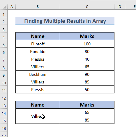
- Drag the Fill Handle down to get the rest of the results of that same lookup value.
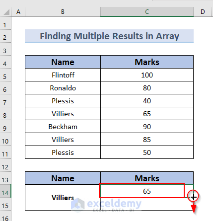
Now you can see the complete Marks.
As this process is not constant for any specific value, you can pick any lookup data in the cell selected (e.g. B14:B15) and the result for that particular data will be auto-updated in the result cell (e.g. C14 and C15).
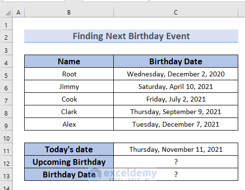
Example 2 – Finding Multiple Results of Upcoming Event Names & Dates
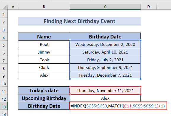
Consider this sample data list of some people’s upcoming birthdays. Let’s find whose birthday is upcoming and on what date based on today’s date using INDEX-MATCH functions.
Steps:
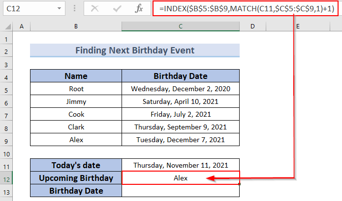
- Enter the following formula in cell C12:
=INDEX($B$5:$B$9,MATCH(C11,$C$5:$C$9,1)+1)
Formula Breakdown
- MATCH(C11,$C$5:$C$9,1)
- Output: 4
- Explanation: The MATCH function finds the position of the lookup value (Cell C11 =Thursday, November 11, 2021) in the array constant ($C$5:$C$9 = the list of the dates). In this example, we didn’t want an exact match, we wanted the MATCH function to return an approximate match, so we set the third argument to 1 (or TRUE).
- INDEX($B$5:$B$9,MATCH(C11,$C$5:$C$9,1)+1) becomes
- INDEX($B$5:$B$9, 4) +1)
- Output: Alex (The name of the person whose birthday is coming next)
- Explanation: The INDEX function takes two arguments to return a specific value in a one-dimensional range. Here, the range $B$5:$B$9 is the first argument and the result that we had from the calculation in the previous section (MATCH(C11,$C$5:$C$9,1)), position 4 is the second argument. That means we are searching the value located in position 4 in the range $B$5:$B$9.
- Press ENTER.
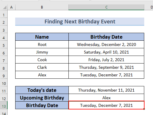
The result is displayed in cell C12.
- To know the Birthday Date, enter the following formula in cell C13:
=INDEX($C$5:$C$9,MATCH(C11,$C$5:$C$9,1)+1)
Formula Breakdown
- INDEX($C$5:$C$9,MATCH(C11,$C$5:$C$9,1)+1) becomes
- INDEX($B$5:$B$9, 4) +1)
- Output: Tuesday, December 7, 2021
- Explanation: The INDEX function takes two arguments to return a specific value in a one-dimensional range. Here, the range $C$5:$C$9 is the first argument and the result that we had from the calculation in the previous section (MATCH(C11,$C$5:$C$9,1)), position 4 is the second argument. That means we are searching the value located in position 4 in the range $C$5:$C$9
- INDEX($B$5:$B$9, 4) +1)
To get the upcoming event date, we just added 1 to the cell position returned by the MATCH function, and it gave us the cell position of the next event date.
- Press ENTER.
The output is displayed in cell C13.
Example 3 – Finding Multiple Results in Separate Columns
Here, we will use the INDEX-MATCH formula with multiple criteria to generate multiple results in multiple columns. We will use the combination of IFERROR, INDEX, ROW, IF, SMALL, COLUMNS, and MIN functions to do the task.
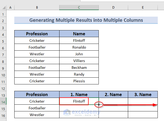
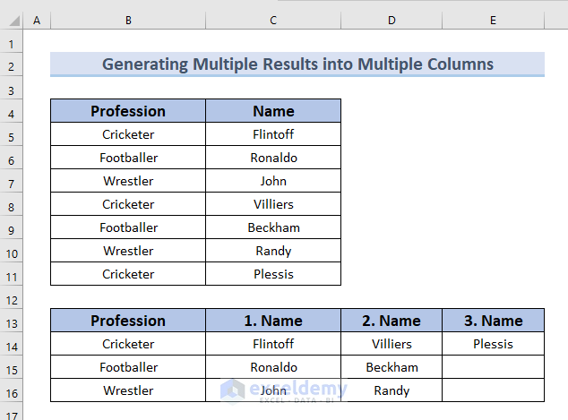
Consider the following dataset, which consists of multiple names of people in three professions. We want to group them based on their profession and to place the names column-wise according to their profession.
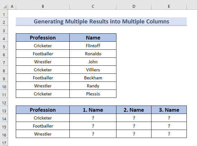
Steps:
- Choose a profession from the data range (B5:B11) and put the data in another cell to use as cell reference number later (e.g., profession Cricketer in cell B14).
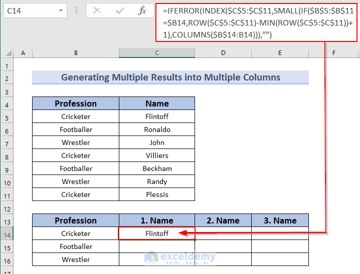
- In another cell that you want as your result cell (e.g. cell C14), enter the following formula:
=IFERROR(INDEX($C$5:$C$11,SMALL(IF($B$5:$B$11=$B14,ROW($C$5:$C$11)-MIN(ROW($C$5:$C$11))+1),COLUMNS($B$14:B14))),"")
Formula Breakdown
- IF($B$5:$B$11=$B14 → becomes
- IF{“Cricketer”, “Footballer”, “Wrestler”, “Cricketer”, “Footballer”, “Wrestler”, “Cricketer”}
- Output: IF{TRUE;FALSE;FALSE;TRUE;FALSE;FALSE;TRUE}
- ROW($C$5:$C$11) → becomes
- Output: {5;6;7;8;9;10;11}
- MIN(ROW($C$5:$C$11) → becomes
- MIN({5;6;7;8;9;10;11})
- Output: 5
- {5;6;7;8;9;10;11}-5 → becomes
- Output: {0;1;2;3;4;5;6}
- {0;1;2;3;4;5;6}+1→ becomes
- Output: {1;2;3;4;5;6;7}
- IF({TRUE;FALSE;FALSE;TRUE;FALSE;FALSE;TRUE},{1;2;3;4;5;6;7})→ becomes
- {1;FALSE;FALSE;4;FALSE;FALSE;7}
- COLUMNS($B$14:B14) → becomes
- Output: 1
- SMALL({1;FALSE;FALSE;4;FALSE;FALSE;7},1) → becomes
- Output:1
- INDEX($C$5:$C$11,1) → becomes
- Output: Flintoff
- IFERROR(Flintoff, “ “) → therefore becomes
- Output: Flintoff
- Press ENTER.
The result is displayed in cell C14.
- Drag the formula toward the right with the Fill Handle tool.
- With C14:E14 selected, drag down the formula with the Fill Handle tool.
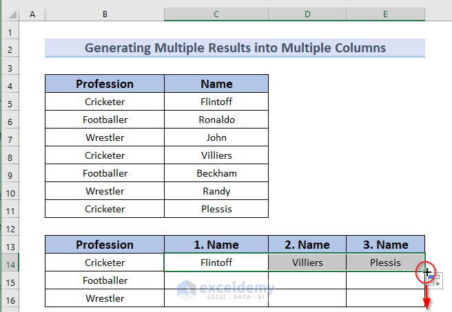
The result in multiple columns is displayed.
Example 4 – Extracting Multiple Values into Separate Rows
Now let’s use the INDEX-MATCH formula to generate multiple results in multiple rows. We will use the combination of IFERROR, INDEX, SMALL, IF, ROW, MIN, and ROWS function for that purpose.
Steps:
- Enter the following formula in cell B14:
=IFERROR(INDEX($C$5:$C$11,SMALL(IF($B$5:$B$11=B$13,ROW(C5:C11)-MIN(ROW(C5:C11))+1),ROWS($B$14:B14))),"")
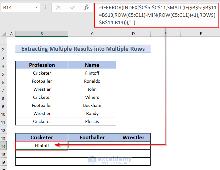
This formula is almost the same as the formula we used in Method 3. The only difference is that we used the ROWS function instead of the COLUMNS function.
- Press ENTER.
The result is displayed in cell B14.
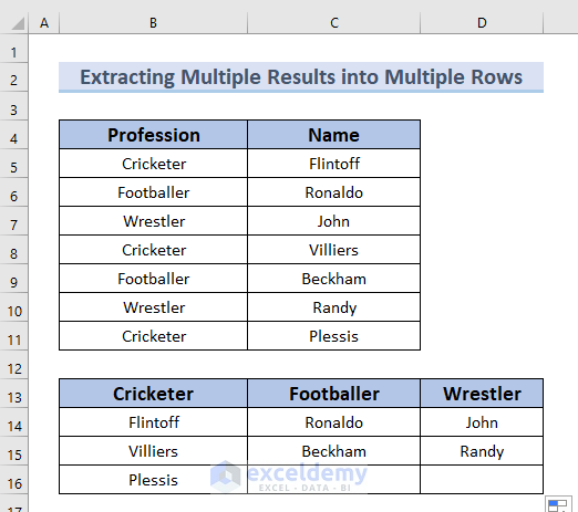
- Drag the formula toward the right with the Fill Handle tool.
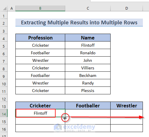
- With B14:D14 selected, drag down the formula with the Fill Handle tool.
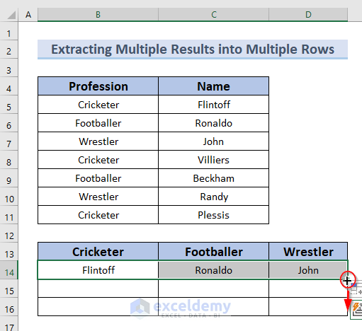
The result in multiple rows is displayed.
Things to Remember
- As the range of the data table array to search for the value is fixed, don’t forget to put the dollar ($) sign in front of the cell reference number of the array table.
- While working with array values, don’t forget to press Ctrl + Shift + Enter on your keyboard while extracting results. Just pressing Enter will work only when you are using Microsoft 365.
- After pressing Ctrl + Shift + Enter, you will notice that the formula bar enclosed the formula in curly braces {}, declaring it as an array formula. Don’t type those brackets {} yourself, Excel automatically does this for you.
Download Practice Workbook
<< Go Back to INDEX MATCH | Formula List | Learn Excel
Get FREE Advanced Excel Exercises with Solutions!

Hi there!
It’s an excellent article, very useful, well explaind steps. I got here because have some issues with Index-Match functions, it is like described under pont 4.: Extract Multiple Results into Separate Rows utilizing INDEX MATCH Functions. Only difference is that I would like to extract the entire row where the match exists. More precisely: I have a lot of data in more columns, one column contains the company names. I would like to extract entire rows for a given company. I don’t know how to implement that difference into Your solution. Can You please give me some advice or guideline?
Thanks in advance!
Thanks ANDREW for your query.
You can check out the following formula that I have applied with the dataset mentioned in the image.
=INDEX(B5:E12,MATCH($B$15,$D$5:$D$12,0),0)
It gives the entire row with the first matched value. But it will not give all the matched rows as output. You can modify the formula using any aggregate function like SMALL to get all the rows at one go.
EMEĞİNİZE SAĞLIK HOCAM =INDEX($C$5:$C$11, SMALL(IF(ISNUMBER(MATCH($B$5:$B$11, $B$14, 0)), MATCH(ROW($B$5:$B$11), ROW($B$5:$B$11)), “”), ROWS($A$1:A1))) OFİS 365 KULLANIYORUM BU FORMÜLÜ OFİS 365 E GÖRE NASILYAPILIR
Dear AHMET KARAASLAN,
Thanks for your comment.
Although the mentioned formula is an array formula, you can use it in Excel for Microsoft 365 without any modifications.
Enter the formula in your required cell and press the Enter key. After that drag down the Fill Handle icon.
Note: This formula can return #NUM! error if any match isn’t found when you use the Fill Handle feature. To avoid this you can combine the IFERROR function with your formula. The modifier formula is:
=IFERROR(INDEX($C$5:$C$11, SMALL(IF(ISNUMBER(MATCH($B$5:$B$11, $B$14, 0)), MATCH(ROW($B$5:$B$11), ROW($B$5:$B$11)),””), ROWS($A$1:A9))),””)
However, if you want to avoid using the Fill Handle feature and want all match results with a single formula, then you can use the FILTER function. This function is only available in Excel for Microsoft 365 and can filter a range based on any given criteria.
To get the same result as the INDEX-MATCH method, apply the following formula in the required cell and press the Enter key.
=FILTER(C5:C11,B5:B11=B14)
I hope this solution will be helpful for you. Let us know your feedback.
Regards,
Seemanto Saha
ExcelDemy