Introduction to Excel INDEX Function
- Objective:
Returns a value of reference of the cell where a specific row intersects with a specified column in a given range.
- Syntax:
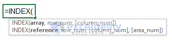
=INDEX(array, row_num, [column_num])
Or,
=INDEX(reference, row_num, [column_num], [area_num])
- Arguments:
array- Range of cells, columns, or rows considered for the values to look up.
row_num- Row position in the array.
column_position- Column position in the array.
reference- Range of arrays.
area_num- Serial number of an array in the reference, if you don’t mention it, it will be considered as 1.
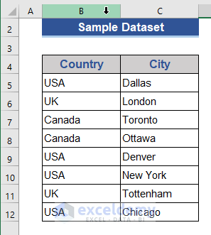
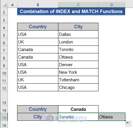
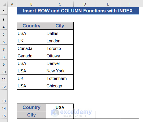
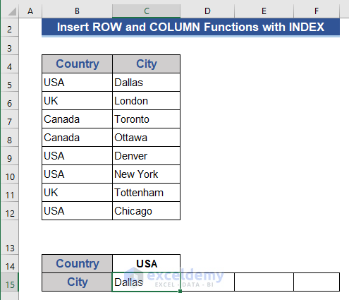
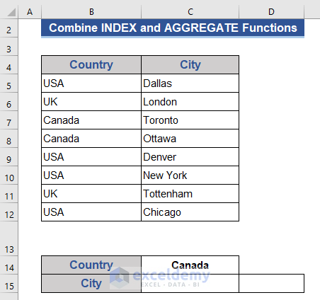
The following dataset showcases names of cities and the corresponding countries.
Use a combination of the INDEX and MATCH functions as a replacement for the LOOKUP function.
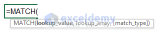
The MATCH function returns the relative position of an item in an array that matches a specified value in a specified order.
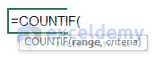
The COUNTIF function counts the number of cells within a range that meet the given condition.
Step 1:
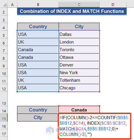
To find the cities in CANADA:
- Enter the following formula in C15.
=IF(COLUMN()-2<=COUNTIF($B$5:$B$12,$C14), INDEX($C$5:$C$12,MATCH($C14,$B$5:$B$12,0)+COLUMN()-3),"")
Step 2:
- Press Enter button and drag the Fill Handle to the right side.
There are 2 cities in CANADA.
Code Breakdown:
- COLUMN()
Provides the column number.
Result: 3
- MATCH($C14,$B$5:$B$12,0)
Searches for a match of C14 in B5:B12.
Result: 3
- COUNTIF($B$5:$B$12,$C14)
Counts how many times C14 is found in B5:B12.
Result: 3
- INDEX($C$5:$C$12,MATCH($C14,$B$5:$B$12,0))
The INDEX operation is performed based on the MATCH function result.
Result: Toronto
Other Formulas to Match & Return Multiple Values Horizontally
1. Combine INDEX with SMALL, IF, ROW, and COLUMN Functions
The INDEX function returns a value or reference of the cell at the intersection of a particular row and column, in a given range.
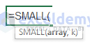
The SMALL function returns the k-th smallest value in a dataset.
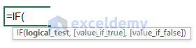
The IF function checks whether a condition is met and returns one value if TRUE, and another value is FALSE.
The COLUMN function returns the column number of a reference.
The ROW function returns the row number of a reference.
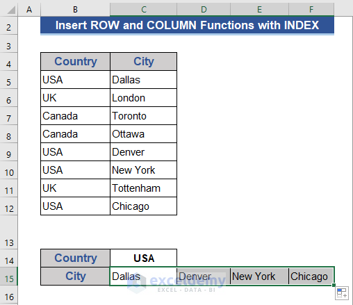
To find all cities in the USA and return their names horizontally:
Step 1:
- Add two rows to the dataset. Enter USA in C14, which will be used as a reference for the formula.
Step 2:
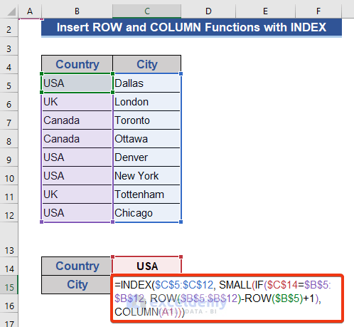
- Go to C15 and enter the following formula.
=INDEX($C$5:$C$12, SMALL(IF($C$14=$B$5:$B$12, ROW($B$5:$B$12)-ROW($B$5)+1), COLUMN(A1)))
Step 3:
- Press Enter to see the result.
Step 4:
- Drag the Fill Handle to the right side.
Code Breakdown
- COLUMN(A1)
returns the column number of A1.
Result: 1
- ROW($B$5)
returns the row number of B5.
Result: 5
- ROW($B$5:$B$12)
provides an array of row numbers in B5:B12.
Result: {5, 6, 7, 8, 9, 10, 11, 12}
- ROW($B$5:$B$12)-ROW($B$5)+1
A subtraction operation is performed, and 1 (one) is added to each subtracted result. This result will be used as an argument for the IF function.
Result: {1, 2, 3, 4, 5, 6, 7, 8}
- IF($C$14=$B$5:$B$12, ROW($B$5:$B$12)-ROW($B$5)+1)
The IF function matches the value of C14 with B5:B12. It returns FALSE when the match is not found.
Result: {1, FALSE, FALSE, FALSE, 5, 6, FALSE, 8}
- SMALL(IF($C$14=$B$5:$B$12, ROW($B$5:$B$12)-ROW($B$5)+1), COLUMN(A1))
The SMALL function provides the smallest number from the array found by applying the IF function.
Result: 1
2. Incorporate the INDEX and AGGREGATE Functions to Return Values Horizontally
To find the name of the cities in CANADA:
The COLUMNS function returns the number of columns in an array or reference.
The AGGREGATE function returns an aggregate in a list or database.
Step 1:
- Enter CANADA in C14.
Step 2:
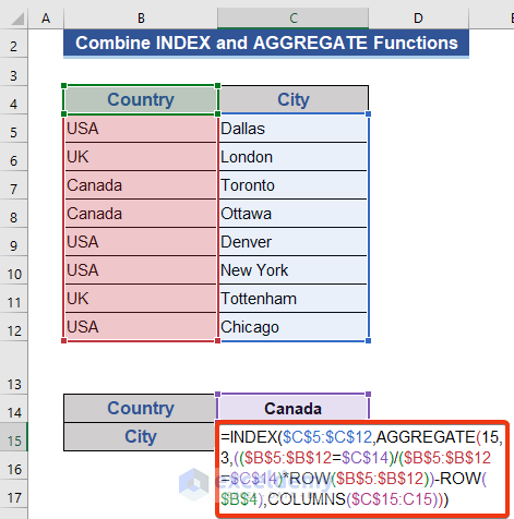
- Enter the formula below in C15.
=INDEX($C$5:$C$12,AGGREGATE(15,3,(($B$5:$B$12=$C$14)/($B$5:$B$12=$C$14)*ROW($B$5:$B$12))-ROW($B$4),COLUMNS($C$15:C15)))
Step 3:
- Press Enter and drag the Fill Handle to the right side.
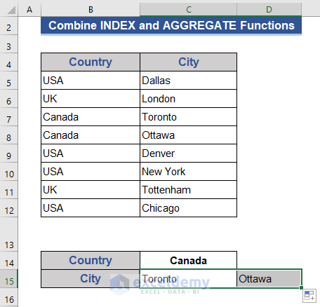
The City names are displayed vertically.
Code Breakdown
- COLUMNS($C$15:C15)
It will return the number of columns from the given array.
Result: 1
- ROW($B$4)
It will return the row number of Cell B5.
Result: 4
- ROW($B$5:$B$12)
It will provide an array of row numbers of Range B5:B12.
Result: {5, 6, 7, 8, 9, 10, 11, 12}
- AGGREGATE(15,3,(($B$5:$B$12=$C$14)/($B$5:$B$12=$C$14)*ROW($B$5:$B$12))-ROW($B$4),COLUMNS($C$15:C15))
In this section, the AGGREGATE function is used to perform a specific operation, which is defined by the 1st argument of the AGGREGATE function. The 1st argument is 15 and defines the SMALL function.
Result: 3
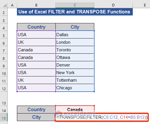
3. Using the TRANSPOSE-FILTER Formula to Return Multiple Values horizontally
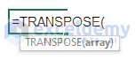
The TRANSPOSE function converts a vertical range of cells to a horizontal range and vice-versa.
The FILTER function filters a range or array.
Step 1:
- In C15, enter the formula below.
=TRANSPOSE(FILTER(C5:C12, C14=B5:B12))
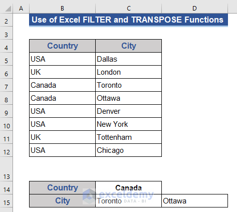
Step 2:
- Press Enter.
Download Practice Workbook
Download the practice workbook.
<< Go Back to INDEX MATCH | Formula List | Learn Excel
Get FREE Advanced Excel Exercises with Solutions!
