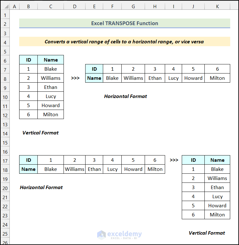
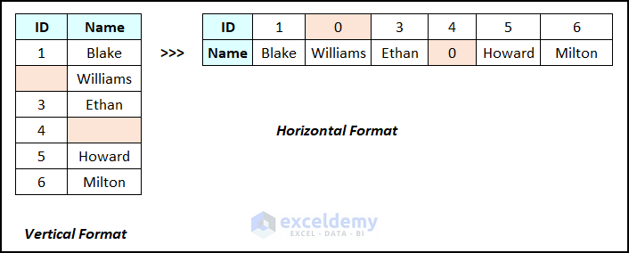
Here’s a quick view of the TRANSPOSE function in the following image.
Introduction to the Excel TRANSPOSE Function
Here are the syntax and the arguments of the TRANSPOSE function in Excel.
- Summary
This function converts a vertical range of cells to a horizontal range or vice versa.
- Syntax
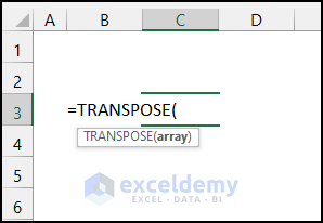
=TRANSPOSE (array)- Arguments
| Argument | Required/Optional | Explanation |
|---|---|---|
| array | Required | Pass the array or range of cells to transpose |
- Version
The TRANSPOSE function is available from Excel 2007. If you have the Microsoft Excel 365 version installed in your system, you can use the dynamic array feature.
How to Use the TRANSPOSE Function in Excel: 3 Suitable Examples
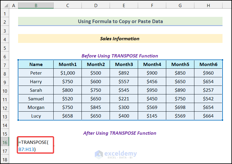
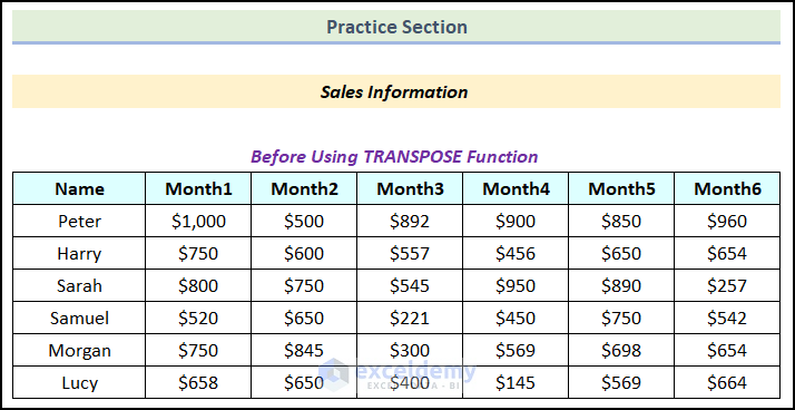
We have a dataset of sales information with salesperson names and the months. The data is all in a vertical format. We’ll rotate the whole dataset into a horizontal formation by converting its rows to columns.
![]()
Example 1 – Copy or Paste Data
Steps:
- Enter the following formula in cell B16.
=TRANSPOSE(B7:H13)The range of cells B7:H13 indicates our entire dataset.
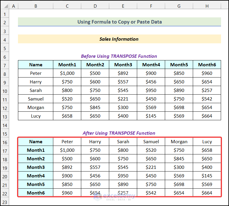
- Press Enter.
All the data will be transformed from a vertical to a horizontal formation, as demonstrated in the following picture.
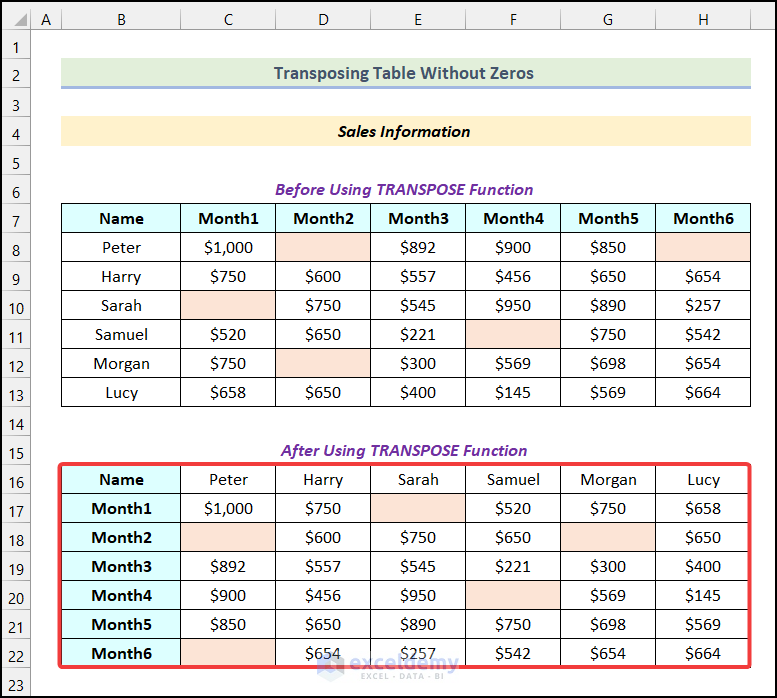
Example 2 – Transpose the Table Without Zeros
When we transpose a data table in Excel, if there are any blank cells on that table, the blank cells are automatically replaced with zeros. This phenomenon is shown in the following image.
We’ll transpose the table without zeros using the TRANSPOSE function. We have some blank cells marked in light orange color.
![]()
Steps:
- Use the following formula in cell B16.
=TRANSPOSE(IF(B7:H13="","",B7:H13))Formula Breakdown
- In the IF function, we are checking if there are any blank cells in the given range or not. If there is any blank cell then print “”(blank cell), otherwise show the values from range B7:H13.
- B7:H13=”” → This is the logical_test argument.
- “” → Indicates the [value_if_true] argument.
- B7:H13 → Refers to the [value_if_false] argument.
- If there are no blank cells, then the TRANSPOSE function transposes the data from the range B7:H13.
- Hit Enter.
![]()
All the blank cells have remained the same as in the source table as shown in the following picture.
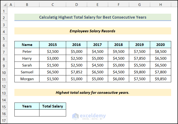
Example 3 – Calculate the Highest Total Salary for the Following Years
We will use the TRANSPOSE function to calculate the highest total salary for consecutive years. We have a dataset of employees’ salary records. All the datasets are organized in a horizontal position. We’ll find out the last four years’ highest salary summation using a formula. We will get the highest total salary for the following years for Morgan.
Steps:
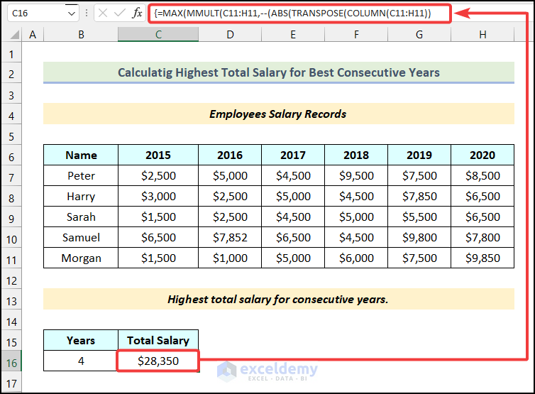
- Enter the following formula in cell C16.
=MAX(MMULT(C11:H11,--(ABS(TRANSPOSE(COLUMN(C11:H11))-COLUMN(OFFSET(C11:H11,0,0,1,COLUMNS(C11:H11)-B16+1))-(B16-1)/2)<B16/2)))Here, the range of cells C11:H11 refers to the salaries of Morgan from the year 2015 to 2020, and cell B16 indicates the number of Years.
Formula Breakdown
- The formula tests the ranges to see if there are enough consecutive columns. The results of those tests (1 or 0) are multiplied by the cell values, to get the total salaries.
- The TRANSPOSE function is used to do all the calculations after converting the rows into columns.
- The MMULT function is used to return the matrix product of two arrays.
- The MAX function is to find out the maximum salary from the given dataset.
- Using two minus signs (—) next to each other causes the formula to convert a return value of “TRUE” into 1 and a return value of “FALSE” into 0.
- Hit Enter.
Alternatives for the TRANSPOSE Function
Alternative 1 – Using the Transpose Option from Paste Options
Case 1.1 – Rotating Data from Rows to Columns
Steps:
- Select the dataset and copy it using the keyboard shortcut Ctrl + C.
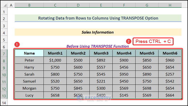
- Select a new location from where you want to start your new table. We have selected cell B16 as our destination cell.
- Go to the Home tab from Ribbon.
- Click on the Paste option from the Clipboard group.
- Choose the Transpose (T) option from the drop-down.
![]()
The data will be formatted vertically as shown in the image below.
![]()
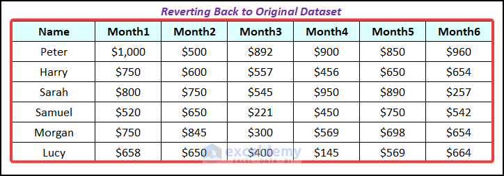
- If you want to go back to the original dataset, copy it again.
![]()
- Select the destination cell. We choose cell B25.
- Use the same procedure to revert to the original dataset.
Case 1.2 – Manipulating Data
We have a dataset of two team players’ names. The dataset is horizontally oriented. We’ll transpose the dataset vertically and rewrite all the names using this formula “Team Name – Player Name”.
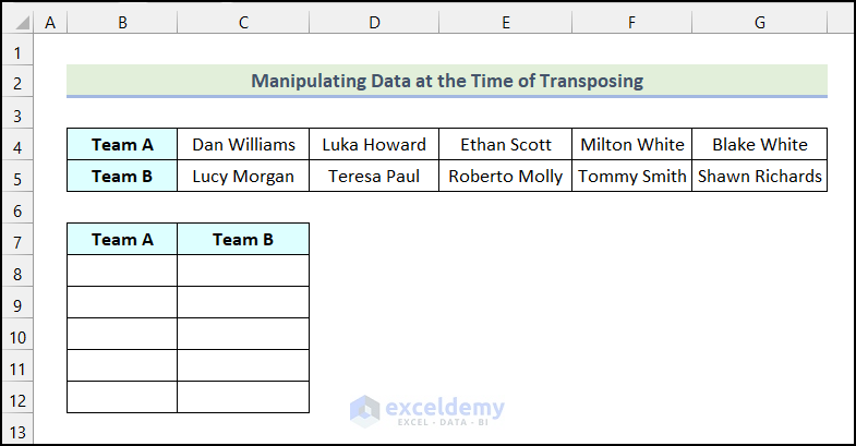
Steps:
- Select the data from Team A only and copy them using the keyboard shortcut Ctrl + C.
![]()
- Select a destination cell where you want to start your new table. We have chosen cell B16 as our destination cell.
- Go to the Home tab from Ribbon.
- Click on the Paste option from the Clipboard group.
- Choose the Paste Link (N) option from the drop-down.

You will have the following output on your worksheet as marked in the image below.
![]()
- Use the keyboard shortcut Ctrl + H to open the Find and Replace dialog box.
- Type = in the Find what box.
- Type “Team A –” in the Replace with field.
- Click on the Replace All option.
![]()
- Excel will pop up a dialog box with a confirmation. Click on OK.
- Click Close.
![]()
- Select the new cells as shown in the following image and press Ctrl + C to copy the cells.
![]()
- Select a destination cell where you want to start your new table. We have chosen cell B8 as our destination cell.
- Go to the Home tab from Ribbon.
- Click on the Paste option from the Clipboard group.
- Choose the Transpose (T) option from the drop-down.
![]()
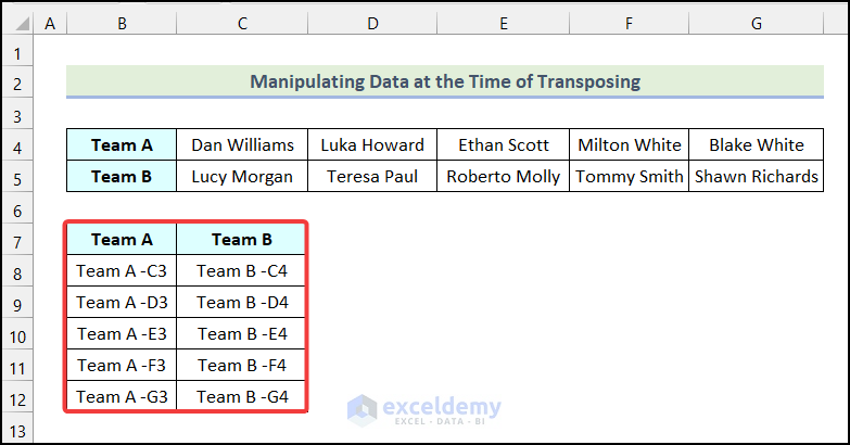
The selected data will be transposed vertically, as demonstrated in the following picture.
![]()
- Follow the same procedure for Team B, and you will get the following output on your worksheet as shown in the image below.
Alternative 2 – Applying the Keyboard Shortcut
Keyboard Shortcut 1
Steps:
- Select the entire dataset and press Ctrl + C to copy the dataset.
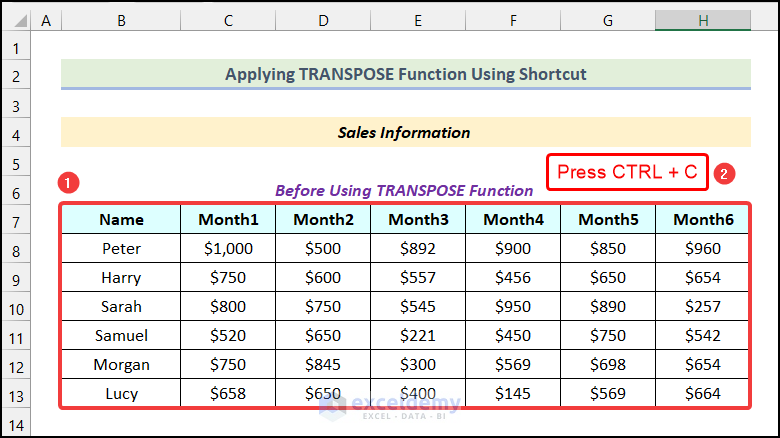
- Select the destination cell.
- Use the keyboard shortcut Alt + H + V + T.
![]()
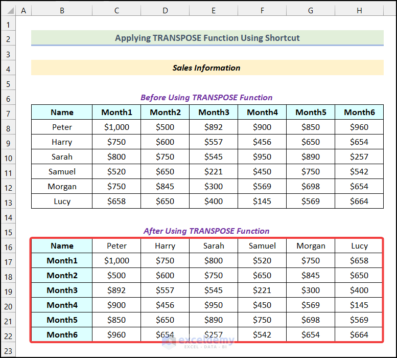
The keyboard shortcut will swap the rows and columns of the original dataset, and you will get the following output, as shown in the following picture.
![]()
Keyboard Shortcut 2
Steps:
- Select the entire dataset and copy it using the keyboard shortcut Ctrl + C.
![]()
- Select the destination cell.
- Use the keyboard shortcut Ctrl + Alt + V. This will open the Paste Special dialog box.
![]()
- Press E.
- Hit Enter.
How to Delete the TRANSPOSE Function in Excel
Steps:
- Use Method 1 to get the following output.
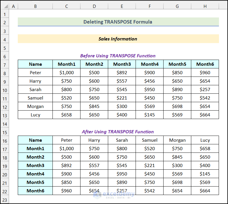
- Select the first cell of the output table.
- Press the Delete key.
![]()
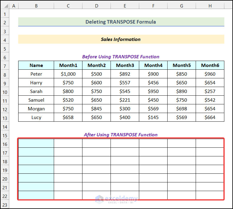
The TRANSPOSE formula will be deleted from the entire output table all at once.
Common Errors While Using the TRANSPOSE Function in Excel
| Common Errors | When They Show |
|---|---|
| Formatting problem | TRANSPOSE does not carry over formatting. |
| #VALUE! | If the formula has not been entered as an array formula. The formula needs to be entered with Ctrl + Shift + Enter |
Things to Remember
- If you also need to transpose the text and cell formatting, then try to use the copy-and-paste options. You can also use the Transpose option to do this. But this may create duplicates. So, if your original cells get changed, then the copies won’t update automatically.
- You don’t have to type the range by hand. After typing =TRANSPOSE(, you can choose the range with your mouse. Simply click and drag from the start of the range to the finish.
- As an array function, the TRANSPOSE does not support modifying part of the array it returns. To edit a TRANSPOSE formula, select the entire range the formula refers to, make the desired change, and press Enter to save the updated formula.
- In the older versions of Excel, you need to press Ctrl + Shift + Enter after writing the TRANSPOSE function.
Practice Section
In the Excel Workbook, we have provided a Practice Section on the right side of the worksheet.
Download the Practice Workbook
<< Go Back to Excel Functions | Learn Excel
Get FREE Advanced Excel Exercises with Solutions!
