Overview of the MAX Function
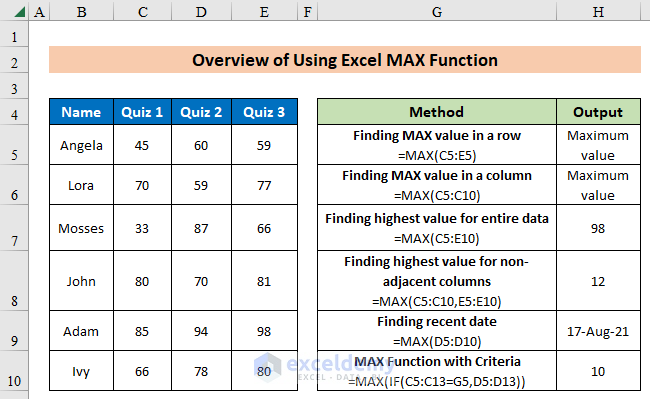
Introduction to MAX Function in Excel
The MAX Function is categorized under Excel STATISTICAL functions. This function returns the largest value in a given list of arguments.
Syntax:
Returns the largest value in a set of values. Ignores logical values and text.
MAX (number1, [number2], ...)Arguments:
| Argument | Required/Optional | Value |
|---|---|---|
| number1 | Required | Reference to a numeric value or range that contains numeric values. |
| [number2] | Optional | Additional numbers, cell references, or ranges of numeric values. |
You can provide up to a maximum of 255 arguments.
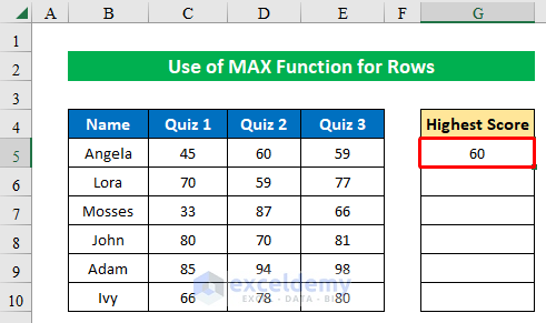
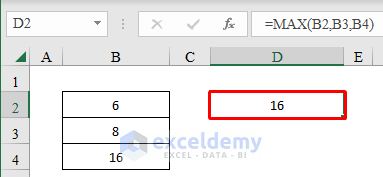
Example 1 – Finding the Maximum Value in a Row
Suppose you have a data table of students with their scores in three quizzes. To find the highest score for each student, insert the formula:
=MAX(C5:E5)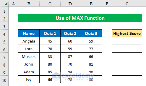
Here, C5:E5 represents the cell reference for the first row.
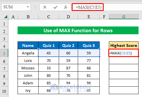
Our formula has provided the highest score for Angela on the quizzes.
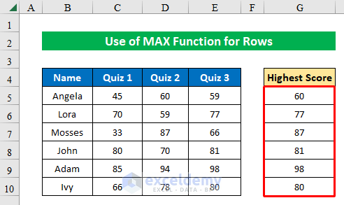
- Drag the Fill Handle to get maximum values for the other rows.
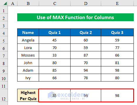
Example 2 – Finding the Maximum Value in a Column
If you want to find the highest score for each quiz (stored in three columns), insert:
=MAX(C5:C10)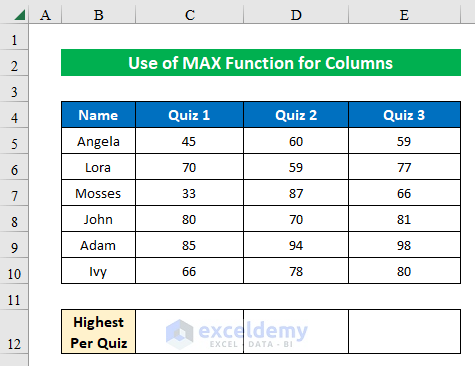
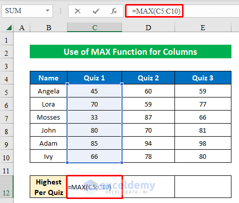
- We have found the highest score for Quiz 1. Drag the Fill Handle to the right to find the largest value for the other columns.
Read More: How to Find Max Value in Range with Excel Formula
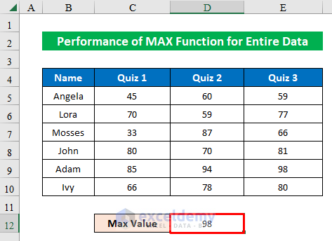
Example 3 – Getting the Highest Value from the Entire Dataset
To find the maximum value from an entire dataset (e.g., prices of items in different shops), insert:
=MAX(C5:E10)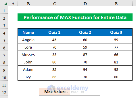
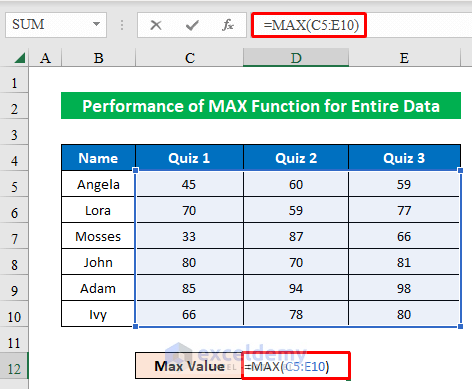
We have found the maximum value in our table.
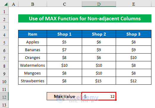
Example 4 – Using the MAX Function for Non-Adjacent Columns
Suppose you want to find the maximum value from non-adjacent columns (e.g., Shop1 and Shop3).
- Insert the following formula:
=MAX(C5:C10,E5:E10)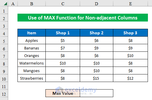
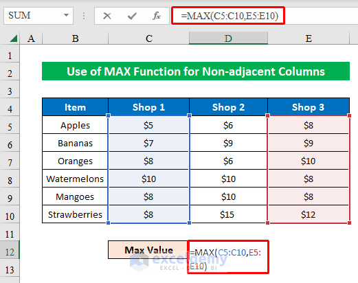
Here we have set the column references separated by a comma (,). The formula provided the maximum value for the two non-adjacent columns.
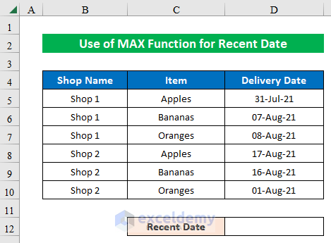
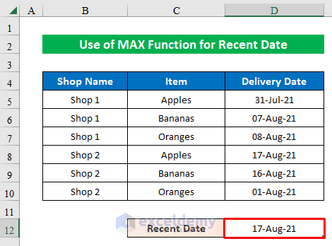
Example 5 – Finding the Most Recent Date
If you have a dataset with delivery dates, use the MAX function to find the most recent date.
- Enter the following formula in cell D12:
=MAX(D5:D10)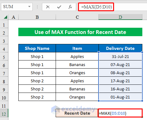
Excel stores dates as sequential serial numbers, with 1 January 1900 as the 1st date (serial number 1).
The MAX function converts the dates into their respective serial numbers and finds the most recent date.
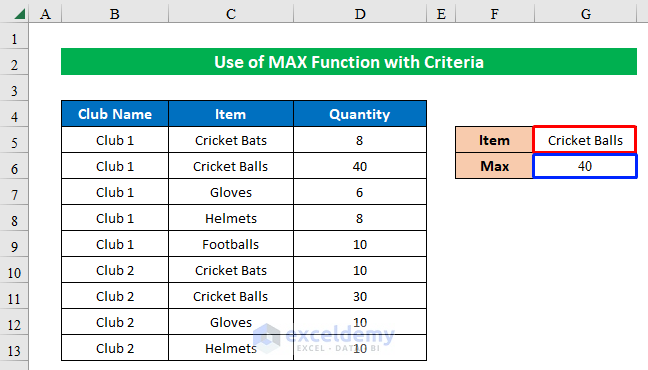
Example 6 – Using the MAX Function with Criteria
Let’s say you have a dataset of sports items and their quantities.
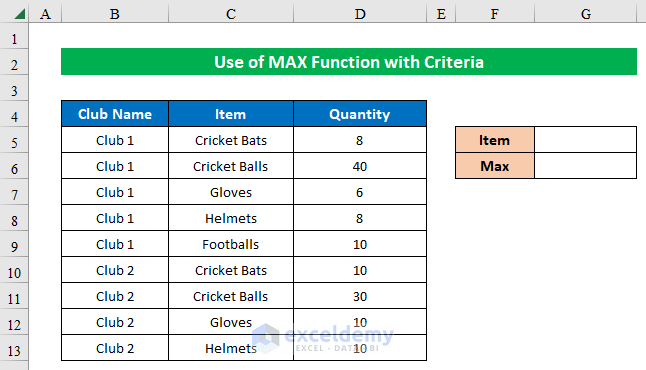
- Set a criteria (e.g., Cricket Bats in cell G5) and insert the formula:
=MAX(IF(C5:C13=G5,D5:D13))-
- We need to set the condition using the IF function.

This array formula checks if the criteria match and triggers the MAX operation.
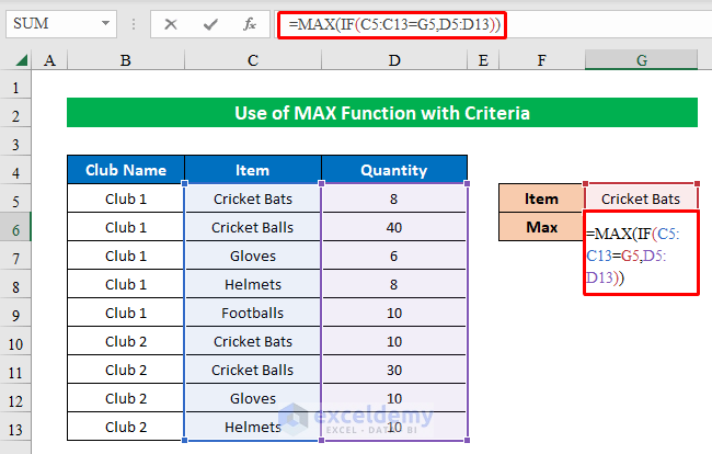
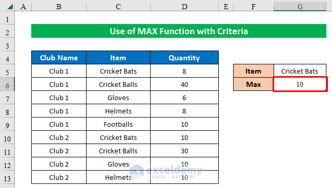
Here we have found the highest quantity of Cricket Bats. If we change the criteria item, the result will be adjusted.
Note: Remember, if you’re using an older version of Excel, press CTRL+SHIFT+ENTER to execute array formulas.
Read More: How to Find Maximum Value in Excel with Condition
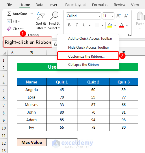
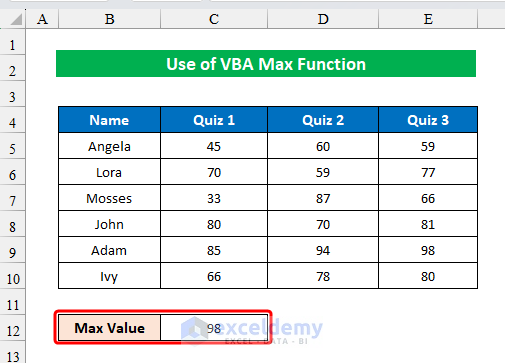
How to Find the Maximum Value with Excel VBA
- Enabling the Developer Tab in Excel:
- If you haven’t already enabled the Developer tab, right-click on any blank area of the Ribbon.
- Select Customize the Ribbon.
-
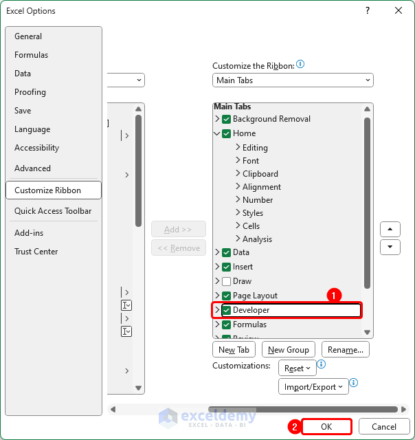
- In the Excel Options dialog box, check the box next to Developer and click OK. The Developer tab will now appear in your ribbon.
- Using VBA Code to Find the Maximum Value:
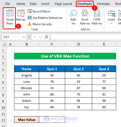
- Go to the Developer tab and click on Visual Basic.
-
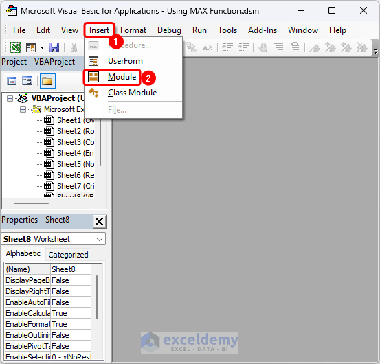
- In the Microsoft Visual Basic for Applications window, go to the Insert tab and select Module from the drop-down.
-
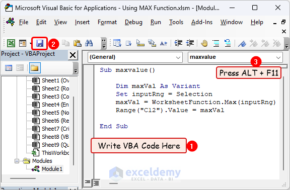
- Enter the following VBA code in the newly created module:
Sub maxvalue()

Dim maxVal As Variant
Set inputRng = Selection
maxVal = WorksheetFunction.Max(inputRng)
Range("C12").Value = maxVal

End Sub-
- Click the Save icon and use the keyboard shortcut ALT + F11 to return to the worksheet.
- Running the Macro:
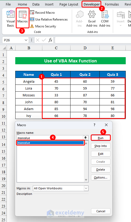
- Select the range of data for which you want to find the maximum value.
- Go to the Developer tab and click on Macros.
- Choose the maxvalue option in the Macro dialog box and click Run.
-
- The maximum value will appear in cell C12.
Quick Notes
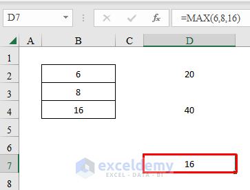
- You can set the Cell References separated by a comma (,). We have inserted 3 cells in the function, and these are separated by a comma.
- You can insert the numbers directly into the function to find the highest value.
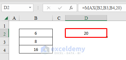
- Numbers can be combined with ranges using a comma (,).
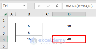
- You can directly input the numbers into the function to get the largest value among them.
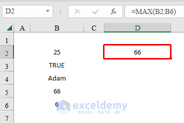
- The MAX function ignores text or Boolean values and focuses on numeric values.
Download Practice Workbook
You can download the practice workbook from here:
Excel MAX Function: Knowledge Hub
- Find Max Value and Corresponding Cell in Excel
- How to Set a Minimum and Maximum Value in Excel
- Excel MIN and MAX in Same Formula
- How to Cap Percentage Values Between 0 and 100 in Excel
<< Go Back to Excel Functions | Learn Excel
Get FREE Advanced Excel Exercises with Solutions!
