Introduction to the INDEX Function
The INDEX function is classified as a Lookup and References function in Excel.
- Syntax
The syntax for the INDEX function is
INDEX(array, row_num, [column_num])
- Arguments
| ARGUMENTS | REQUIREMENT | EXPLANATION |
|---|---|---|
| array | Required | This is an array element or a cell range. |
| row_num | Required | This is the row location from which a referral will return. |
| column_num | Optional | This is the column position from which a referral will be returned. |
- Return Value
Returns a value or references to a value from a table or range of values.
Introduction to the MATCH Function
The MATCH function examines a cell for a particular match and returns its precise location within the range.
- Syntax
The syntax for the MATCH function is
MATCH(lookup_value, lookup_array, [match_type])
- Arguments
| ARGUMENTS | REQUIREMENT | EXPLANATION |
|---|---|---|
| lookup_value | Required | This means that the value is in a range that will be checked. |
| lookup_array | Required | This means the range within which the value will be searched. |
| match_type | Optional | Used to specify the function’s match type. In most cases, it is a numerical value. There are three sorts of matches that may be used:
To find an exact match, enter 0. 1 to discover the greatest value less than or equal to the search value. -1 to discover the least value greater than or equal to the search value. |
- Return Value
Returns the value that represents a lookup array location.
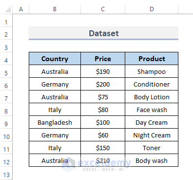
Dataset Introduction
To utilize the functions for returning multiple values into one cell, we are using the following dataset. The dataset represents a small local business that sells products after importing them from different countries. It contains Countries in column B from where they import the products, the Price of each product in column C, and the Product name in column E.
Suppose we need to extract all the products imported from a specific country.
Excel INDEX MATCH to Return Multiple Values in One Cell: Step-by-Step Procedures
Step 1 – Apply INDEX and MATCH Functions to Return Multiple Values
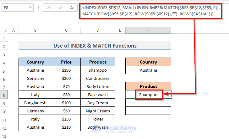
Let’s extract all the products imported from Australia.
- Select the cell where you want to put the formula.
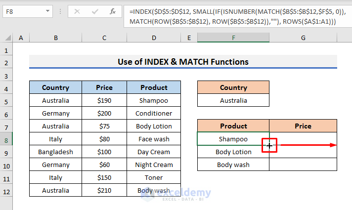
- Put this formula into that selected cell.
=INDEX($D$5:$D$12, SMALL(IF(ISNUMBER(MATCH($B$5:$B$12,$F$5, 0)), MATCH(ROW($B$5:$B$12), ROW($B$5:$B$12)),""), ROWS($A$1:A1)))- Pess the Enter key.
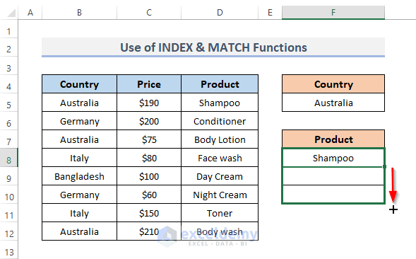
- Drag the Fill Handle down to duplicate the formula over the range or double-click on the Plus (+) symbol.
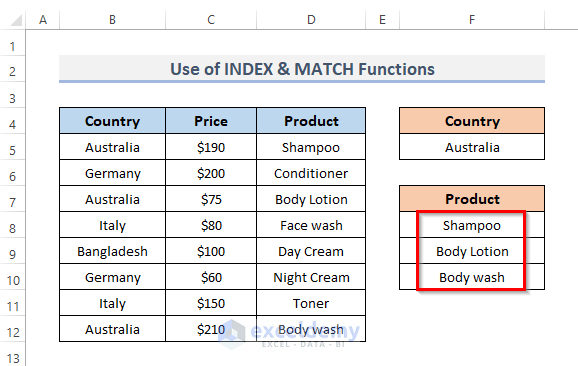
- Here’s the result in cell range F8:F10.
How Does the Formula Work?
- ROWS($A$1:A1): In this section, we use cell A1 as a starting point.
- ROW($B$5:$B$12)): This part shows cells B5 through B12 are selected.
- MATCH(ROW($B$5:$B$12), ROW($B$5:$B$12)),””): The portion looks for values that match exactly in the range (B5:B12) and returns them.
- (MATCH($B$5:$B$12,$F$5, 0)): This section looks for values that match the value of cell F5 in the range (B5:B12).
- ISNUMBER(MATCH($B$5:$B$12,$F$5, 0): Determines whether or not the matched values in the range (B5:B12) are numbers.
- IF(ISNUMBER(MATCH($B$5:$B$12,$F$5, 0)): The line means that if there are any matching values in the range (B5:B12), the IF formula returns.
- SMALL(IF(ISNUMBER(MATCH($B$5:$B$12,$F$5, 0)),MATCH(ROW($B$5:$B$12), ROW($B$5:$B$12)),””),ROWS($A$1:A1)): For each array, this function returns the lowest matching value.
- INDEX($D$5:$D$12,SMALL(IF(ISNUMBER(MATCH($B$5:$B$12,$F$5, 0)),MATCH(ROW($B$5:$B$12), ROW($B$5:$B$12)),””),ROWS($A$1:A1))): Finally, this formula searches the array (D5:D12) for matched values and returns them in cell (F8:F10).
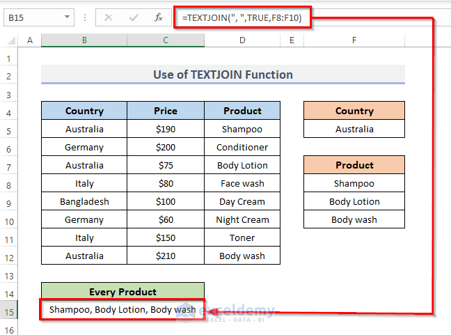
Step 2 – Excel TEXTJOIN or CONCATENATE Function to Put Multiple Values in One Cell
- Select the cell where you want to put the multiple-valued result into one cell.
- Enter this formula into the cell.
=TEXTJOIN(", ",TRUE,F8:F10)- Press Enter to see the result.
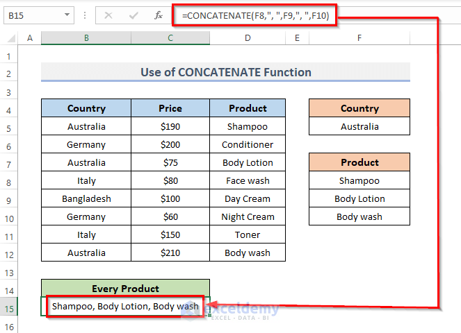
- Instead of using the TEXTJOIN function, you can also use the CONCATENATE function in that selected cell. Enter this formula into that cell.
=CONCATENATE(F8,", ",F9,", ",F10)- Press Enter. As a result, this formula will show the result for putting the multiple values into one cell.
Download the Practice Workbook
<< Go Back to INDEX MATCH | Formula List | Learn Excel
Get FREE Advanced Excel Exercises with Solutions!

Hello, Can you use this same methodology to create a dropdown list? Didn’t seem to work when I tried.
Hello, MICHAEL!
https://www.exceldemy.com/excel-dependent-drop-down-list-multiple-words/
Please, check this article!
How do get the result to go across cells instead of down. Eg I would need the result to go into cells F8-G8 in the example. I have a spreadsheet with over 6000 rows
Hi ROBYN,
Thanks for your comment. I am replying to you on behalf of Exceldemy. To get the results across the cells, you need to drag the Fill Handle to the right side and make the necessary changes if needed. Suppose, we also need the Price along with the products. We can get the prices using some steps. Let me show you the process in the steps below.
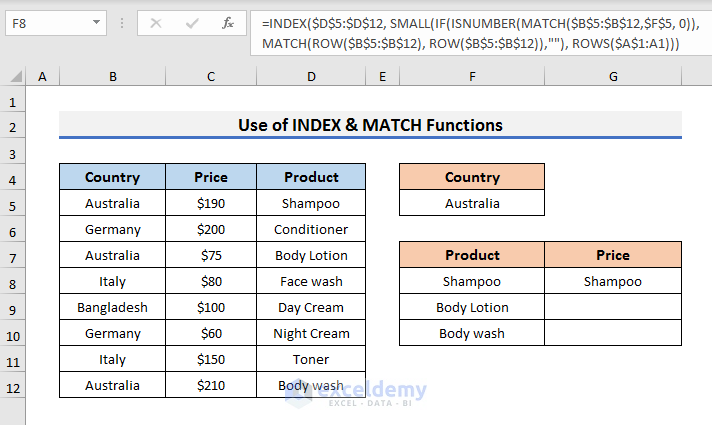
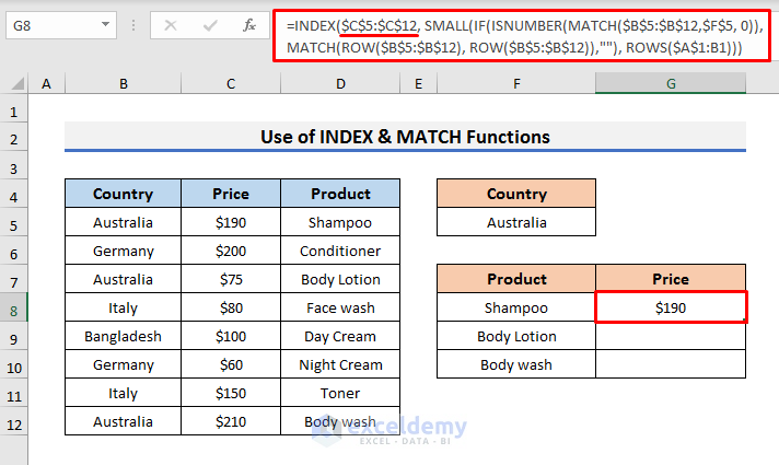
STEPS:
1. Firstly, put the cursor on the bottom corner of Cell F8. It will turn into a small plus sign.
2. Now, drag the Fill Handle to the right to Cell G8.
3. It will show the same result and formula because the range D5:D12 is locked.
4. Now, select Cell G8 and go to the Formula Bar.
5. Type
$C$5:$C$12in place of$D$5:$D$12because Column C contains the prices.6. Press Enter.
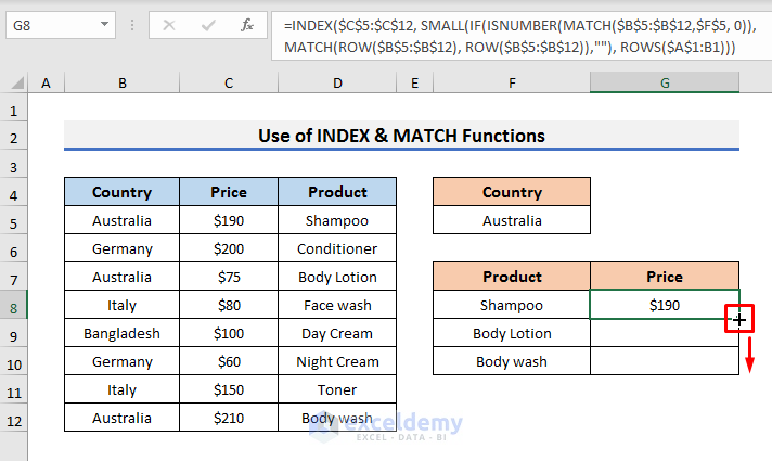
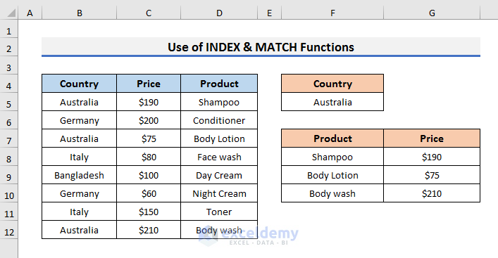
7. After that, drag the Fill Handle down.
8. Finally, you will see the prices of the products.
To know more about copying formulas across cells you can check the article below.
Copy Formula Across Cells
I hope this will help you to solve your problem. Please let us know if you have other queries.
Thanks!
Hello, Robyn! You can copy the formula into the cell where you need it.
Did you find a way?
Hi JESSICA,
Thanks for your comment. I am replying to you on behalf of Exceldemy. You can check the comment thread for the answer. Also, to know more about copying formulas across cells, you can check the link below.
Copy Formulas Across Cells
Thanks!
If you use COLUMNS instead of ROWS for the last function you can drag across multiple rows
Hi BEN,
Thanks for your comment. I am replying to you on behalf of Exceldemy. To know more about copying formulas across cells, you can check the link below.
Copy Formulas Across Cells
Thanks!