In this article, we’ll demonstrate how to use the INDEX & MATCH functions to find the minimum or smallest value in Excel, using the Microsoft 365 version.
Introduction to INDEX & MATCH Functions
INDEX Function
Formula Syntax:
or,
Activity:
Gives a value from the given array at the intersection cell of the provided row and column numbers.
Example:
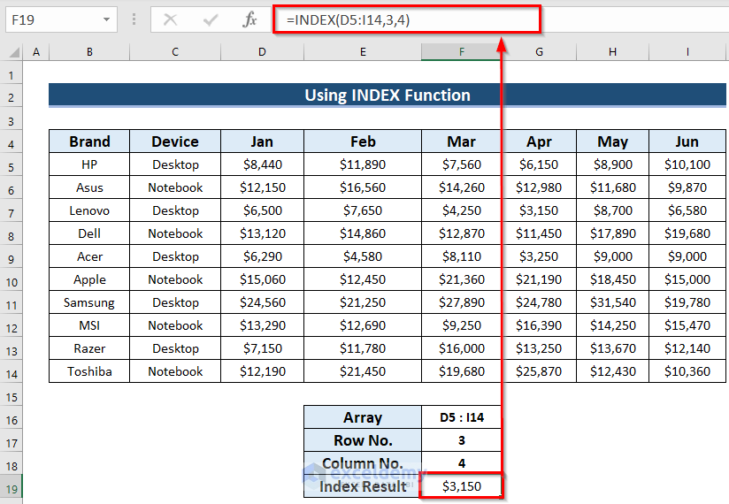
Suppose we have a table with names of different brands, device types, and the related sales prices for 6 months. We want to know the sales price at the intersection of the 3rd row & 4th column in the array of selling prices.
Steps:
- In Cell F19, enter:
=INDEX(D5:I14,3,4)- Press ENTER to get the result.
Here, the 4th column in the array represents the selling prices of all devices for April & the 3rd row represents the Lenovo Desktop category, at their intersection in the array D5:I14. Thus, the formula will return the selling price of Lenovo Desktop in April.
MATCH Function
Formula Syntax:
Activity:
Gives the relative position of an item in a given array that matches a certain value in a fixed order.
Example:
Using the same dataset, we’ll find the position of the month of June in the month headers.
Steps:
- In cell F17, our formula will be:
=MATCH(F16,D4:I4,0)- Press ENTER to return the column position of the month of June in the month headers, namely 6.
- Change the name of the month in cell F16 to return the related column position of that month.
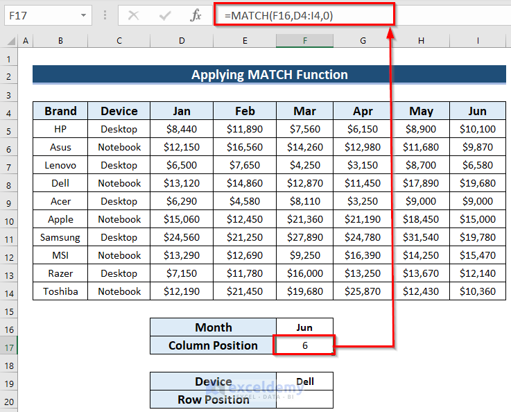
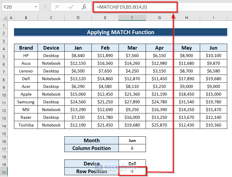
And if we want to know the row position of the brand Dell from the names of the brands in Column B, then the formula in cell F20 will be:
=MATCH(F19,B5:B14,0)Here, B5:B14 is the range of cells in which the name of the brand will be looked for. If you change the brand name in cell F19, you’ll get the related row position of that brand from the selected range of cells.
INDEX-MATCH Formula to Find Minimum Value in Excel: 4 Suitable Approaches
Method 1 – Combining INDEX, MATCH & MIN Functions to Get Minimum Price
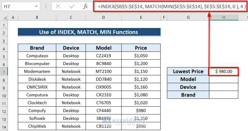
Using our sample dataset from above, let’s find which price is the lowest in Column E.
Steps:
- In cell H7, enter the following:
=INDEX($B$5:$E$14, MATCH(MIN($E$5:$E$14), $E$5:$E$14, 0 ), 4 )- Press ENTER to return the lowest price.
How Does This Formula Work?
- The MIN function extracts the smallest or minimum value from the range of Cells E5:E14.
- The MATCH function finds the row position of that minimum value.
- Within the INDEX function, B5:E14 is the entire array where our data extraction functions are applied. The other arguments are the row number and column number.
- ‘4’ is the column number since the price list is present in the 4th column of the selected array.
- The INDEX function now extracts the data from Column E based on the row and column criteria.
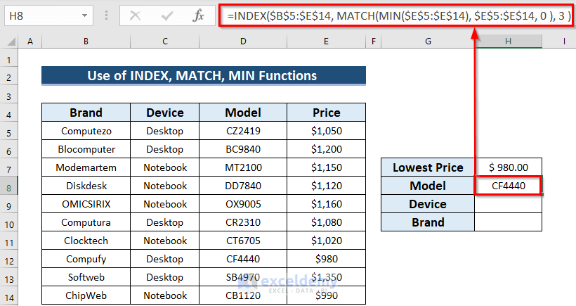
Now, we’ll find out the model name or number corresponding to the lowest price.
- In our output cell H8, the formula will be:
=INDEX($B$5:$E$14, MATCH(MIN($E$5:$E$14), $E$5:$E$14, 0 ), 3 )Here, 3 is the column number for the INDEX function as all model names are present in the 3rd column of the selected array.
Furthermore, in cell H9, we’ll find out the type of device matching the lowest price. Here, the column number will be 2.
- So, the formula in cell H9 will be:
=INDEX($B$5:$E$14,MATCH(MIN($E$5:$E$14),$E$5:$E$14,0),2)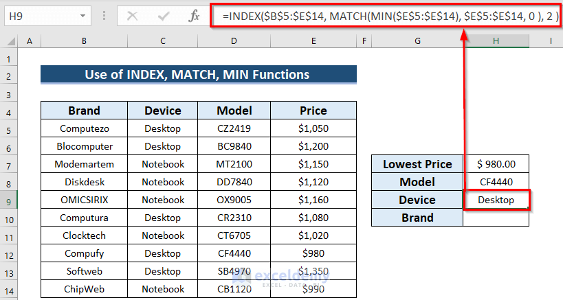
Finally, we’ll determine which computer brand is offering the lowest price.
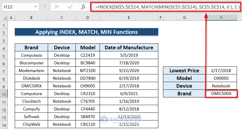
- In cell H10, the formula will be:
=INDEX($B$5:$E$14,MATCH(MIN($E$5:$E$14),$E$5:$E$14,0),1)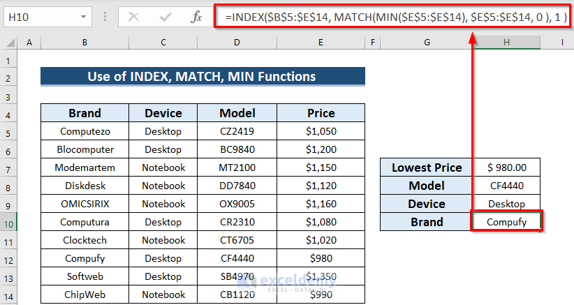
Method 2 – Combining INDEX, MATCH & MIN Functions to Find Earliest Date
By using a similar formula, we can also find out the earliest date from a range of cells containing dates. In our modified dataset below, the Date of Manufacture column has been added to assign dates. We’ll find out which date is the earliest.
Steps:
- Select cell H7 and enter:
=INDEX($B$5:$E$14,MATCH(MIN($E$5:$E$14),$E$5:$E$14,0),4)- Press ENTER to return the earliest date.
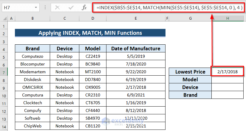
As the dates are present in the 4th column of the selected array, so we’ve set the column number of the INDEX function to 4. Now, if we wanted to extract the model name, device type & brand name for that particular date of manufacture, we would simply change the column number for the INDEX function accordingly.
Method 3 – Combining INDEX, MATCH & AGGREGATE Functions to Find Minimum Value with Multiple Criteria
We’ll use the AGGREGATE function for finding minimum values with multiple criteria.
Formula Syntax:
Or,
Arguments:
- function_num – A list of 19 functions with serial numbers will appear when typing the function. Select the serial number of the function required.
- options – Provides options to ignore errors or numerical data.
- array – The selected array or range of cells on which the formula will work.
- [k] – Serial number or position in the array based on the return values.
Activity:
Returns an aggregate in a list or database.
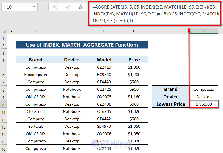
In Column B some names appear multiple times. Suppose we want to find the lowest price for a specified brand device, such as the desktop of Computezo brand.
Steps:
- In cell H10 enter:
=AGGREGATE(15, 6, E5:INDEX(E:E, MATCH(1E+99,E:E))/ ((B5:INDEX(B:B, MATCH(1E+99,E:E ))=H8)*(C5:INDEX(C:C, MATCH(1E+99,E:E ))=H9)),1)- Press ENTER to return the lowest price of Computezo desktop.
How Does This Formula Work?
- Inside the array, 15 is the Function Number that is assigned to the SMALL function.
- 6 is the Option Number that ignores any Error Values.
- In the 3rd argument, a complex array is established. The dividend or numerator part returns an array with all prices from the list, which looks like:
- {1050;1200;980;950;1160;960;1020;980;1350;1050;1070;1020}
- The divisor or denominator has two parts which both work with logical functions. The 1st part looks for the brand name Computezo in Column B and the 2nd part looks for a desktop device in Column D. Then the converted (TRUE=1, FALSE=0) and numerical logic values are multiplied alongside these two parts. The resultant array returns as:
- {1;0;0;0;0;1;0;0;0;0;1;0}
- All the prices found from the dividend will be divided by these logical values found from the divisor, which returns:
- {1050;#DIV/0!;#DIV/0!;#DIV/0!;#DIV/0!;960;#DIV/0!;#DIV/0!;#DIV/0!;#DIV/0!;1070;#DIV/0!}
- Finally, the AGGREGATE function ignores all the Error Values and extracts the smallest value from the array.
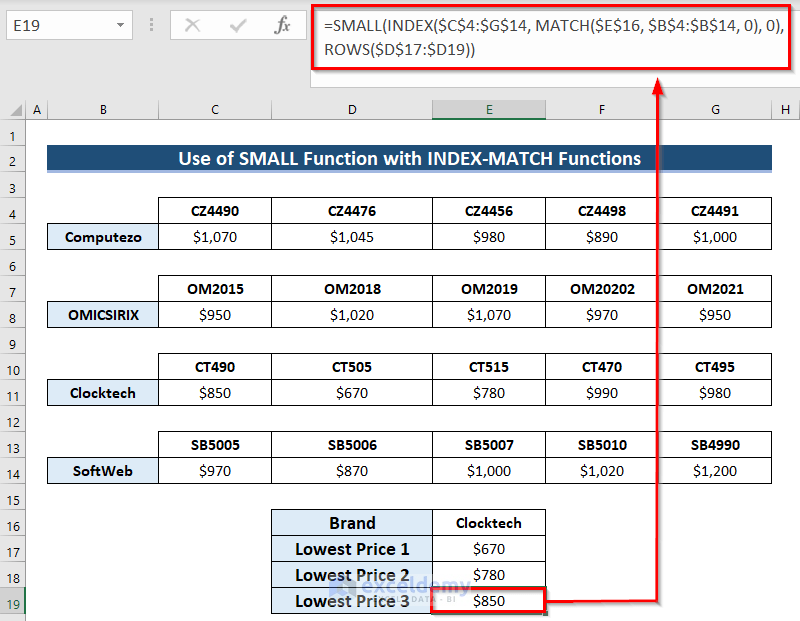
Method 4 – Fusing SMALL Function with INDEX-MATCH to Find Minimum or Smallest Three
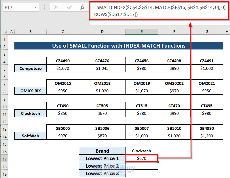
In our final method, we’ll apply the SMALL function, which extracts the smallest value from a range of cells or an array based on the defined position or serial of the smallest value. In the dataset below, prices of different models of 4 computer brands are listed. we’ll find the lowest three prices of a specific brand, Clocktech.
Steps:
- In cell E7, our formula will be:
=SMALL(INDEX($C$4:$G$14, MATCH($E$16, $B$4:$B$14, 0), 0), ROWS($D$17:$D17))- Press ENTER to return the lowest price for the Clocktech brand.
- To get the 2nd & 3rd lowest prices, drag the Fill Handle icon down to cells E18 and E19.
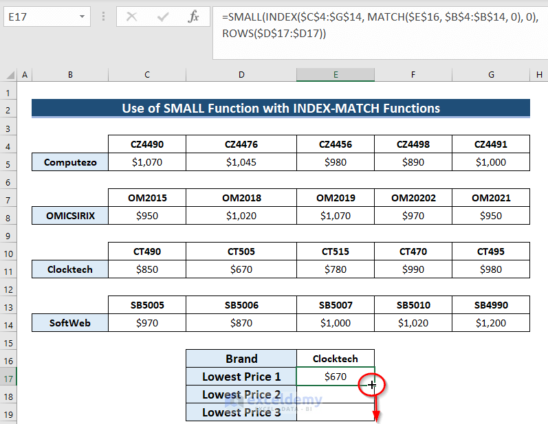
As a result, we have the 3 lowest prices of the Clocktech brand. Furthermore, in cell E16, if you change the brand name, you’ll find the lowest 3 prices of that brand.
How to Use VLOOKUP Function to Find Minimum Value in Excel
Instead of an INDEX-MATCH formula, we can use the VLOOKUP function along with the MIN function to find a minimum value in Excel. One important consideration when using the VLOOKUP function is that the reference column must be the first column in the lookup table. Accordingly, we’ve modified our dataset to place the Price column first. Let’s find the lowest price.
Steps:
- Enter the following formula in cell H7:
=VLOOKUP(MIN(B5:B14),B5:E14,1,FALSE)- Press ENTER to return the value.

How Does This Formula Work?
VLOOKUP(lookup_value,table_array,col_index_num,[range_lookup])
- MIN(B5:B14) will extract the lowest value, which will be the lookup_value for the VLOOKUP function.
- B5:E14 is the table_array in which the lookup_value will be sought in the leftmost column.
- 1 is the column index from which the value is to be returned.
- FALSE denotes an exact match.
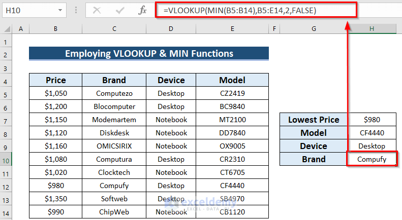
- To find the corresponding model name. we just have to change the column index number in the formula, which is 4:
=VLOOKUP(MIN(B5:B14),B5:E14,4,FALSE)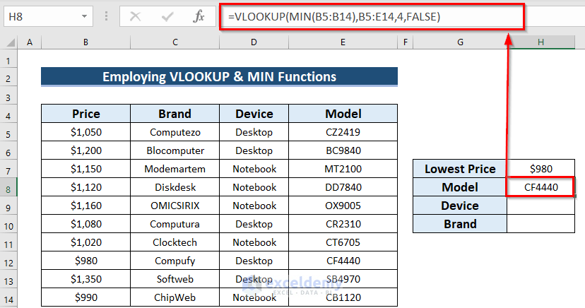
- Similarly, change the column index number to get the device and brand name.
Download Excel Workbook
<< Go Back to INDEX MATCH | Formula List | Learn Excel
Get FREE Advanced Excel Exercises with Solutions!
