[Fixed!] INDEX MATCH Not Returning Correct Value in Excel (5 Reasons)

INDEX Function in Excel

The INDEX function returns the value of a cell at the intersection of a particular row and column in an array or range.

• Syntax

INDEX (array, row_num, [col_num], [area_num])

• Arguments

array: the constant array or the cell range.

row_num: the row number from the desired array.

[col_num]: the column number of the desired array (optional).

[area_num]: the range at the intersection of row_num and col_num (optional).

MATCH Function in Excel

The MATCH function looks for a specific value in an array or range and returns the relative position of that value within it.

• Syntax

MATCH (lookup_value, lookup_array, [match_type])

• Arguments

lookup_value: the value that we search in a range or array.

lookup_array: the array where we search for the lookup_value.

[match_type]: the type of match we want (optional). Set 0 for an exact match, 1 for the greatest value which is less than or equal to the lookup_value, and -1 for the smallest value which is greater than or equal to the lookup_value.

INDEX and MATCH Combination

The combination of INDEX and MATCH functions is one of the most powerful combinations in Excel.

The INDEX function looks up a value in a certain range. Then the MATCH function extracts the matched value using the given arguments.

INDEX MATCH Not Returning Correct Value in Excel: 5 Possible Reasons with Solutions

Let’s try to look up a value in our sample dataset using INDEX MATCH and solve the problems we may face.

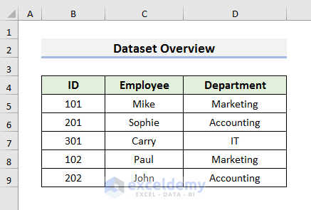
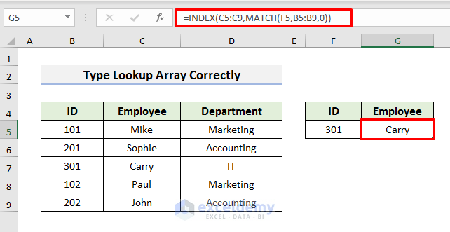
Reason 1 – Exact Match Is Not Correct

INDEX MATCH will not return the correct value if you do not provide any match type. You need to provide the exact match type when you are using this formula. Suppose, we want to extract the name of the employee in cell G5 given the ID number in cell F5. If we change the ID number, the name of the employee will also be updated automatically. For that purpose, we have written the formula below:

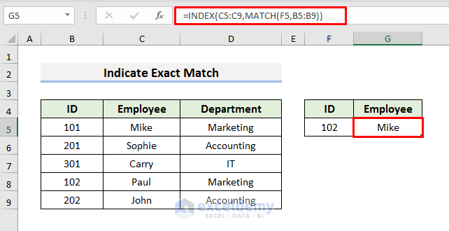
In this case, the formula should have extracted Paul in cell G5. But, it has shown Mike which is not the correct value.

Solution – Indicate Exact Match Correctly

In the above formula, we did not use any match type in the third argument inside the MATCH function. We need to enter 0 in the third argument of the MATCH function.

STEPS:

• Select Cell G5.
• Enter this new formula instead of the previous one:

• Hit Enter to see the correct result.

The only difference between this formula and the previous one is that we have used 0 to indicate the exact match in the third argument inside the MATCH function.

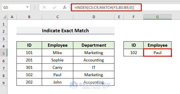
Reason 2 – Blank Cells in the Range or Lookup Array

In cell G5, the correct result is displayed. We can see from the original dataset that 301 is the ID number of Carry.

But if blank cells are inserted in the original dataset, cell G5 will subsequently show an incorrect result.

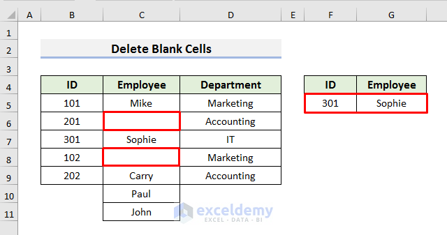
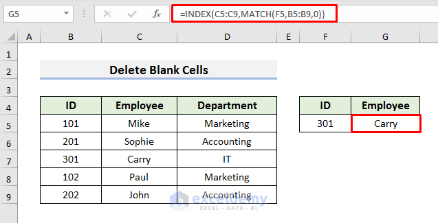
Solution – Delete Blank Cells

STEPS:

• Select the blank cell and right-click on it. A context menu will appear.
• Select Delete from the context menu.

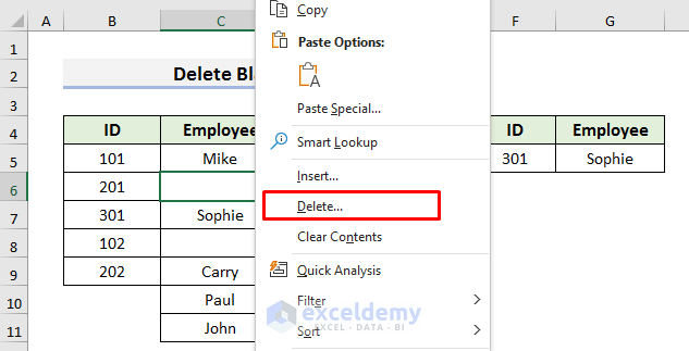
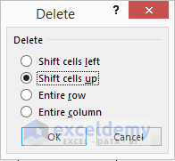
• A message box will appear. Select Shift cells up and click OK to proceed.

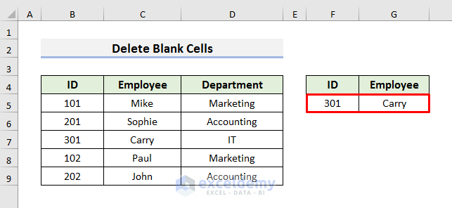
The formula will now return the correct value.

Reason 3 – Table and Range Don’t Correspond

When you are using a table, you need to be extra careful. Suppose, we have converted our previous dataset into a table and named it EmployeeID. Now, we write the formula below to extract the employee name from the given ID:

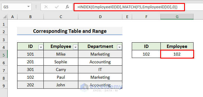
The formula is incorrectly showing the ID number instead of the employee name. The first argument of the INDEX MATCH is EmployeeID[ID], which represents the column that has the header ID in the table named EmployeeID.

Solution – Match Corresponding Table and Range

STEPS:

• Select Cell G5 and enter the formula below:

• Press Enter to see the correct result.

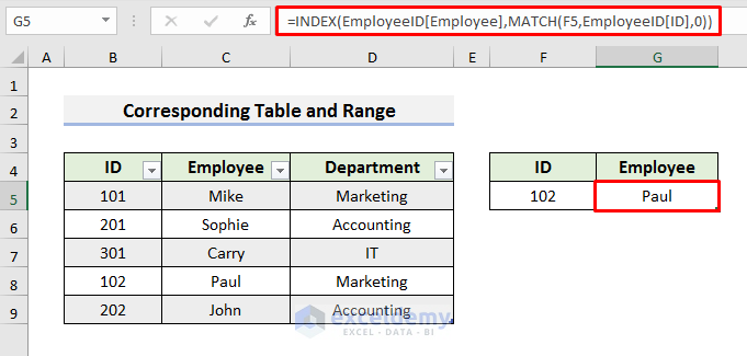
The trick was to use EmployeeID[Employee] instead of EmployeeID[ID], and enter the name of the table correctly.

Reason 4 – Wrong Lookup Array Is Provided

To understand the problem, take a look at the picture below. Here, we used the formula below in cell G5:

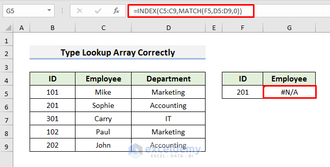
The formula is showing the #N/A error in cell G5. But, if we enter IT in cell F5, we will see a value in cell G5. The wrong lookup array is being referenced.

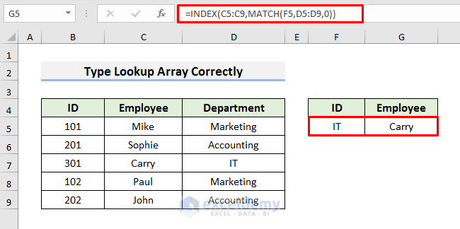
Solution – Enter the Lookup Array Correctly

In our case, our lookup value is the ID number that is situated in the B5:B9 array. So B5:B9 is our correct lookup array.

STEPS:

• Select cell G5 and enter the formula:

• Press Enter to see the result.

The main difference between this formula and the previous one is that we have written B5:B9 in place of D5:D9.

Reason 5 – Reference Is Not Locked

This problem occurs when you drag the INDEX MATCH formula down or across.

We have dragged the formula down in the picture below. We can see the correct results in cells G6 to G8, but some are wrong, and in cell G9, we have a #N/A error. This happens when the reference is not locked. The arrays will move along the direction of the dragging and produce wrong results or errors.

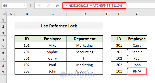
Solution – Use Reference Lock Correctly in Formula

To get rid of the problem, you need to lock your reference. In Excel, we use the dollar ($) sign to lock any cell or reference.

STEPS:

• Select cell G5 and enter the formula below:

• Press Enter to see the result.

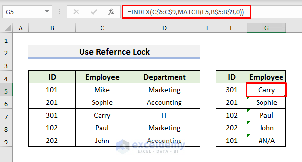
• Drag the Fill Handle down to see the correct values.

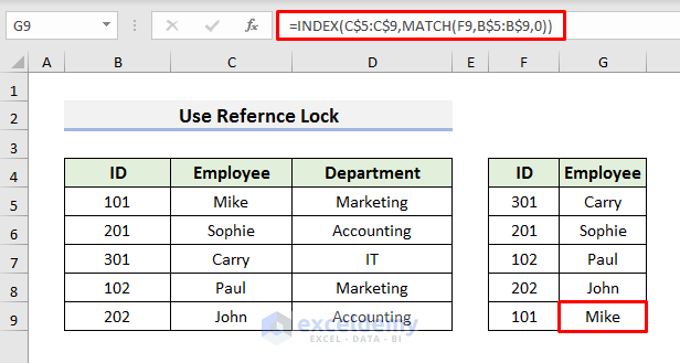
Always lock the references carefully. If you want to drag the formula across, you need to lock the column index too by placing a dollar ($) sign before the column index.

Download Practice Book

<< Go Back to INDEX MATCH | Formula List | Learn Excel