Method 1 – Using the INDIRECT Function in a Table
Steps:
- Select cell C15.
- Enter the following formula:
=INDEX(INDIRECT("Table1["&B15&"]"),MATCH($C$14,Table1[Full Name],0))- Click Enter.
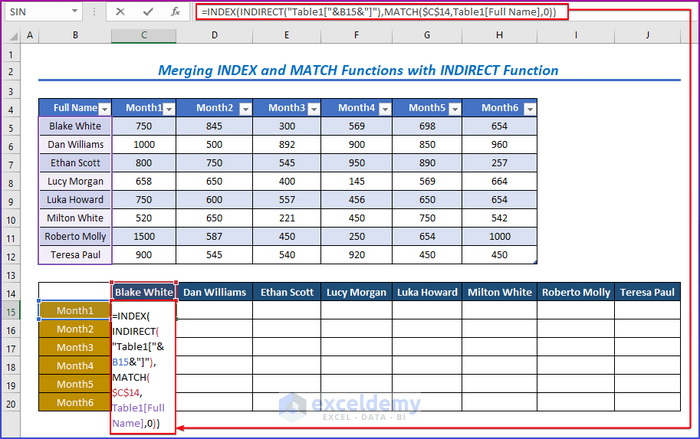
Formula Breakdown
- The sales table is mainly a pivot table. Which is named Table 1.
- MATCH($B$12, Table1[Full Name],0): Using this part, we check for any matched names in the Name column. And 0 is used for exact matching.
- INDIRECT(“Table1[“&A13&”]”) Here, in the INDIRECT function, “Table1[“&A13&”]” is the reference text.
- Using the INDEX function, we are extracting data for the matched rows.
- The result for the first person in cell C15.
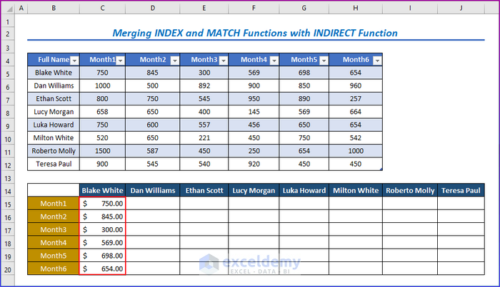
- Use the Fill Handle tool and drag it down from cell C15 to cell C20.
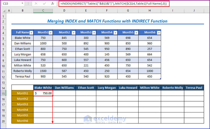
You will get the following results.
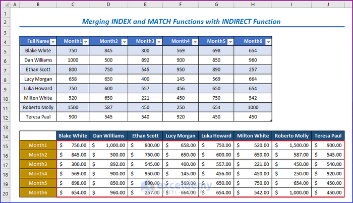
- Copy the formula for the other columns.
You will get all the results in the below image.
Method 2 – Combining INDIRECT, INDEX, and MATCH Functions to Find Data
Steps:
- Choose cell D16.
- Enter the following formula in the cell:
=INDEX(E5:E12-INDIRECT("G5"),MATCH(D15,B5:B12,0))- Press Enter after choosing any name you want to enter in cell D15.
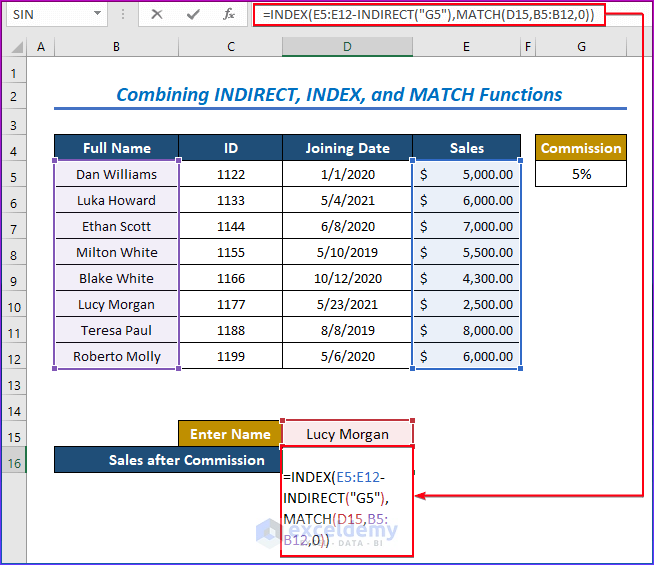
Formula Breakdown
- The primary output value for the INDEX function is E5:E12-INDIRECT(“G5”), which is obtained and evaluated after matching.
- The INDIRECT function in Excel protects Cell References with the syntax INDIRECT(“G5”).
- MATCH(D15, B5:B12, 0) checks the dataset for a match with the specified name.
- Lastly, the INDEX function then extracts the resultant value.
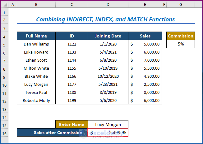
You will get the following result.
Method 3 – Nesting INDIRECT, INDEX, and MATCH Functions to Extract Data from Different Worksheets
Steps:
- We need three different worksheets with data named Data1, Data2, and Data3. All the worksheets contain the Product Name, Quantities, Branch, and Price.
- The first data set includes Product Name, Quantities, Branch, and Price.
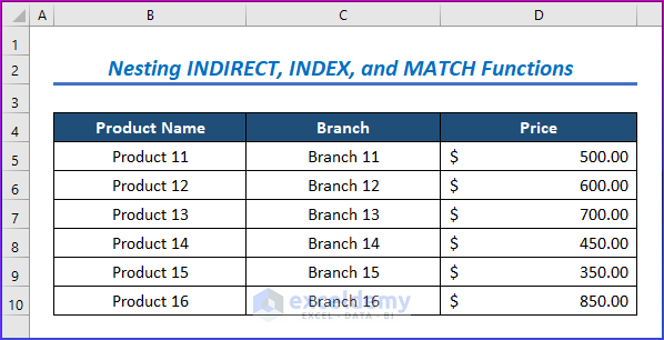
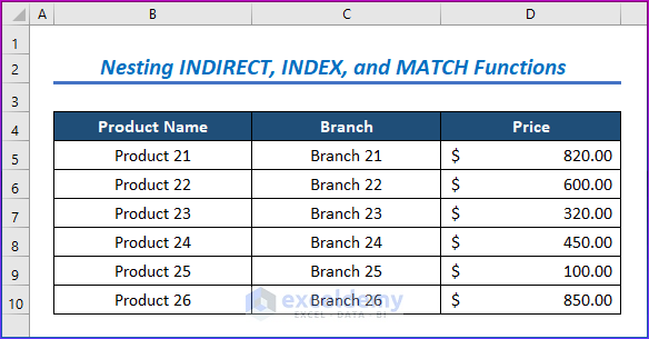
- The second data set included Product Name, Quantities, Branch, and Price (Product 21 – Product 26).
- The third data set includes Product Name, Quantities, Branch, and Price (Product 31 – Product 36).
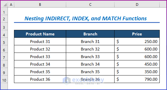
The task is to search Product Prices by entering their Tab Name, Product Name, and Branch.
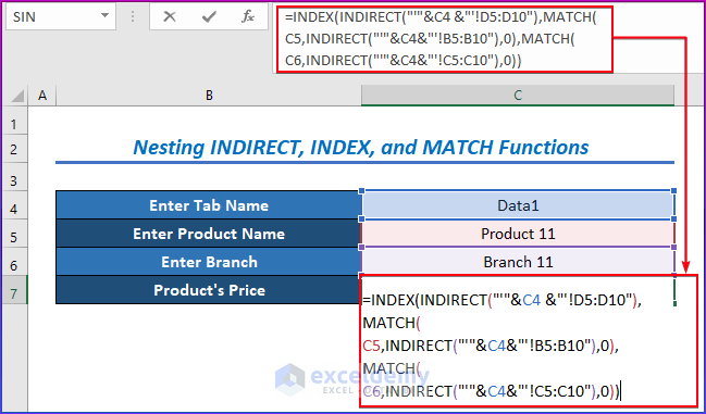
- Enter the following formula in cell C7 after entering all the above-mentioned names.
=INDEX(INDIRECT("'"&C4 &"'!D5:D10"),MATCH( C5,INDIRECT("'"&C4&"'!B5:B10"),0),MATCH( C6,INDIRECT("'"&C4&"'!C5:C10"),0))- Press Enter.
Formula Breakdown
- MATCH(C6,INDIRECT(“‘”&C4&”‘!C5:C10”),0) is the column_num argument of the INDEX function which results in 1.
- MATCH(C5,INDIRECT(“‘”&C4&”‘!B5:B10”),0) is the row-num argument of the INDEX function, which results in 1.
- INDIRECT(“‘”&C4 &”‘!D5:D10”) works as the array argument of the INDEX function, which results in the whole data set of the sheet or tab named Data1.
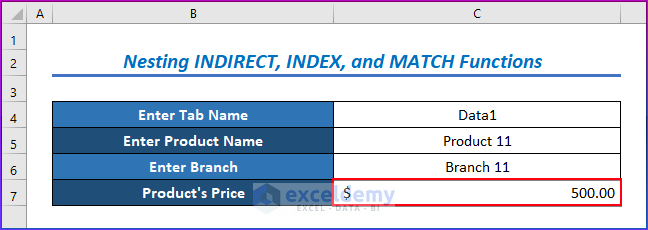
- The INDEX function will figure out the data of the matched cell, which is $ 500.
You will get the following result, as in the below image.
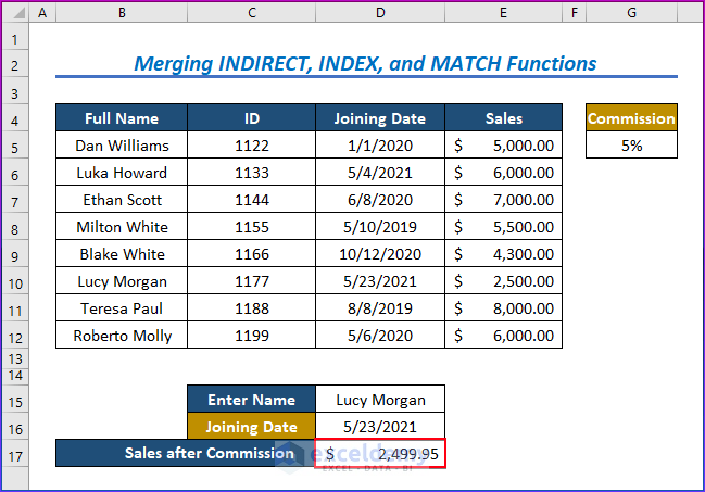
Method 4 – Merging INDIRECT, INDEX, and MATCH Functions to Search Data Based on Condition
Steps:
- Choose cell D17.
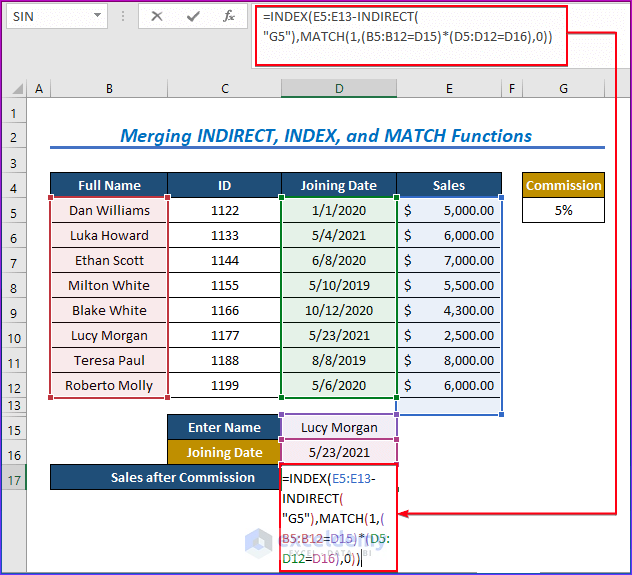
- Enter the following formula after entering any name and joining date:
=INDEX(E5:E13-INDIRECT("G5"),MATCH(1,(B5:B12=D15)*(D5:D12=D16),0))- Press Enter.
Formula Breakdown
- The primary output value for the INDEX function is E5:E13-INDIRECT(“G5”), which is obtained and evaluated after matching. The Excel INDIRECT function locks Cell References using INDIRECT(“G5”).
- MATCH(1,(B5:B12=D15)*(D5:D12=D16),0) searches the dataset for a match with the specified name.
- Lastly, the INDEX function then extracts the resultant value.
The image below shows the result.
Things to Remember
| Common Errors | When they show |
|---|---|
| #VALUE error in INDEX | All ranges must be on one sheet or the INDEX function returns a #VALUE error. |
| Case-Sensitive | The MATCH function is not case-sensitive. |
| #REF! in INDIRECT | All the parameters used in the INDEX formula in Excel, such as Row_num, Column_num, and Area_num, should refer to a cell within the array defined; otherwise, the INDEX function on Excel will return #REF! error value. |
Download the Practice Workbook
Download the following Excel workbook to practice.
<< Go Back to INDEX MATCH | Formula List | Learn Excel
Get FREE Advanced Excel Exercises with Solutions!
