This is an overview of the INDEX function.
The sample dataset contains 2 columns: Country and City.
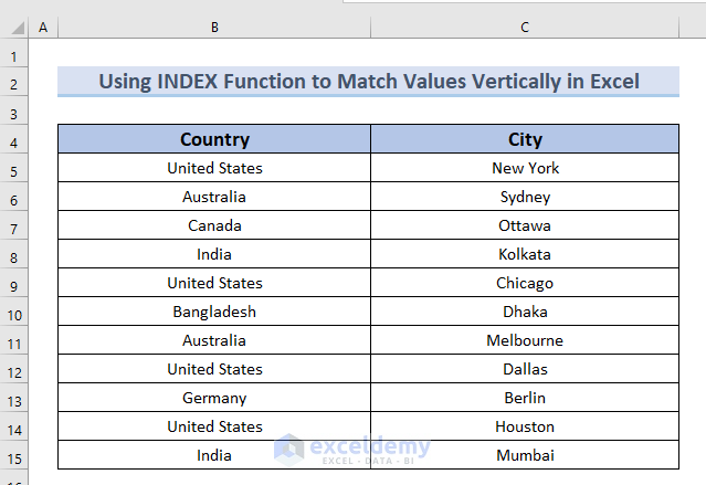
Method 1 – Using the INDEX Function to Match and Return Multiple Values Vertically
Steps:
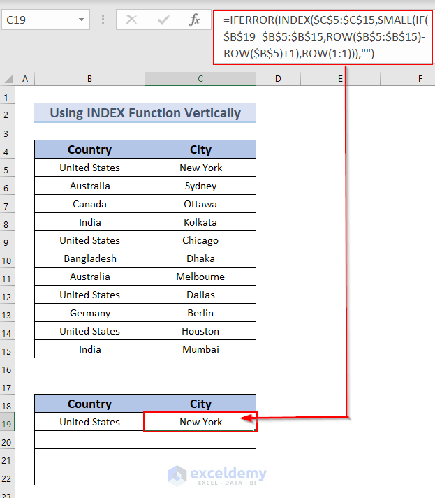
Enter the following formula in C19.
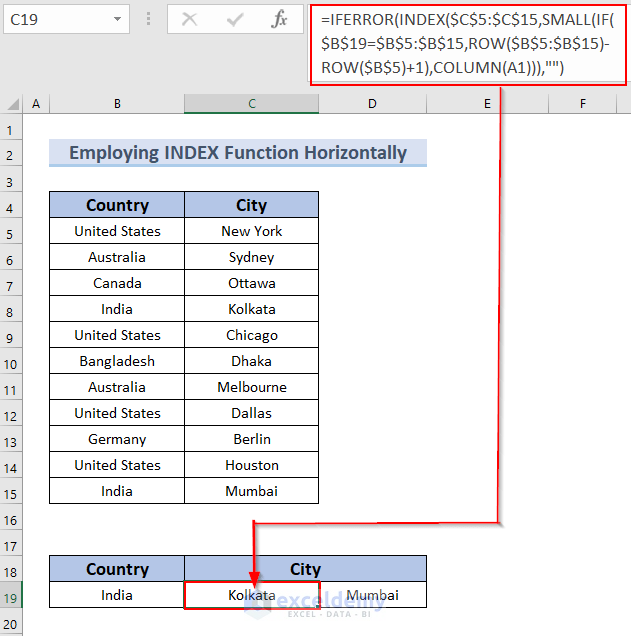
=IFERROR(INDEX($C$5:$C$15,SMALL(IF($B$19=$B$5:$B$15,ROW($B$5:$B$15)-ROW($B$5)+1),ROW(1:1))),"")
Formula Breakdown
- $C$5:$C$15 is the range.
- $B$19 is the lookup criteria.
- $B$5:$B$15 is the range for the criteria.
- ROW(1:1) indicates that the value will be returned vertically.
- Output: New York
- Press ENTER.
You will get see the first city in the United States in C19.
- Drag down the Fill Handle to see the result in the rest of the cells.
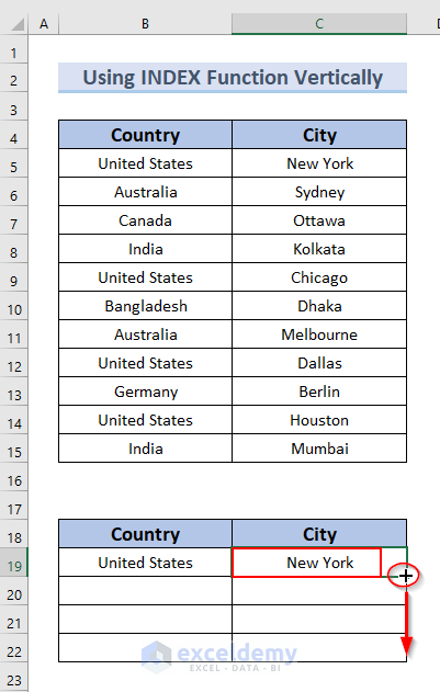
This is the output.
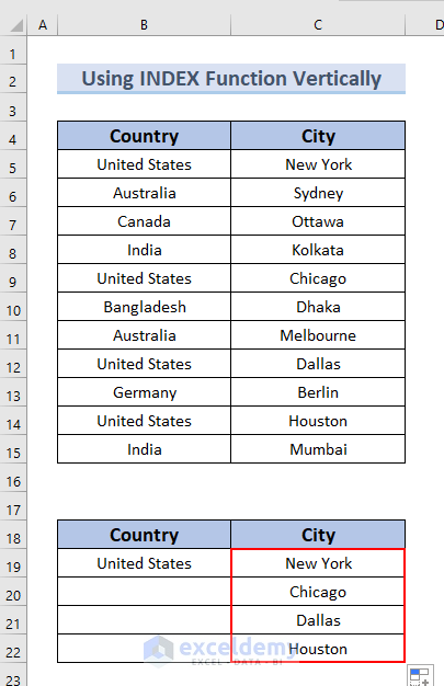
You can apply the formula to other countries:
- Enter the country name in B19, it will automatically return the cities in the City column.
- Observe the GIF.
To use the INDEX function to match and return multiple values horizontally, use the following formula:
- Drag the formula to the right to see the City column.
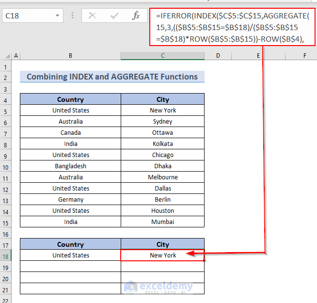
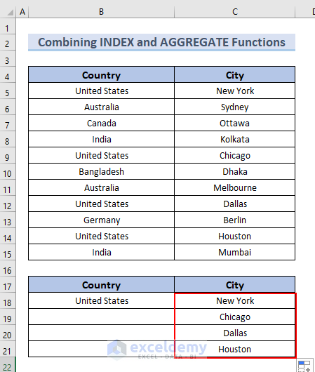
Method 2 – Combining the INDEX and the AGGREGATE Functions to Match and Return Multiple Values Vertically
Steps:
- Enter the following formula in C18.
=IFERROR(INDEX($C$5:$C$15,AGGREGATE(15,3,(($B$5:$B$15=$B$18)/($B$5:$B$15=$B$18)*ROW($B$5:$B$15))-ROW($B$4),ROWS($C$18:C18))),"")
Formula Breakdown
- $C$5:$C$15 is the range for the value.
- $B$18 is the lookup criteria.
- $B$5:$B$15 is the range for the criteria.
- Output: New York
- Press ENTER.
You will see the first city in the United States in C18.
- Drag down the Fill Handle to see the result in the rest of the cells.
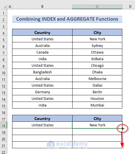
- This is the output.
How to Use the TEXTJOIN Function to Return Multiple Values in a Cell in Excel
Steps:
- Enter the formula in C18.
=TEXTJOIN(“,”,TRUE,IF(B5:B15=B18,C5:C15,””))
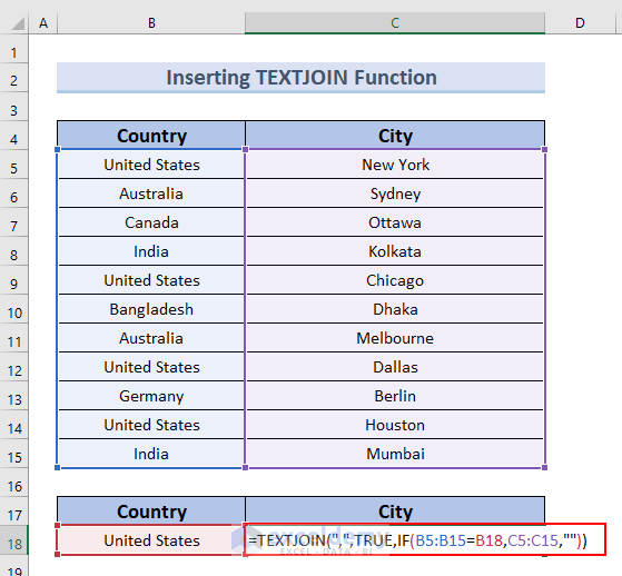
Formula Breakdown
- B18 is the Criteria.
- B5:B15 is the Range to match the criteria.
- C5:C15 is the Range of values.
- TRUE ignores all empty cells.
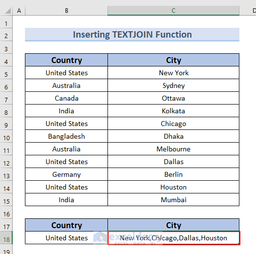
- TEXTJOIN(“,”,TRUE,IF(B5:B15=B18,C5:C15,””)) → it becomes
- Output: New York,Chicago,Dallas,Houston
- Press ENTER.
You can see the result in C18.
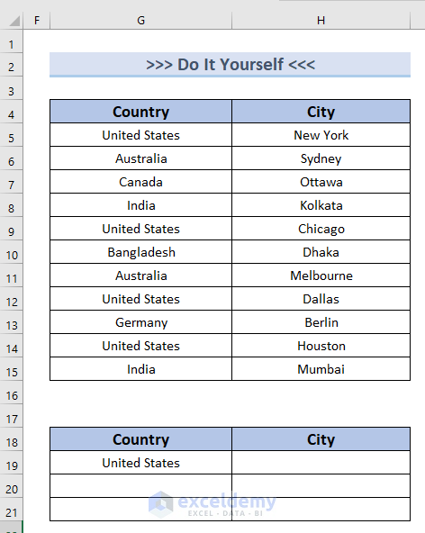
Practice Section
Download the Excel file and practice.
Download Practice Workbook
<< Go Back to INDEX MATCH | Formula List | Learn Excel
Get FREE Advanced Excel Exercises with Solutions!

Hey there and many thanks for sharing your knowledge so generously.
I have a complicated problem and lost in solutions, hoping you can help me with:
Making it simple (hopefully), I want to count all occurrences of a certain code (there are different codes in table cells) in certain rows of the table. rows are selected based on a code in first column of the table.
Hope I could describe it clear enough.
Many thanks in advance
Thanks dar for finding the article helpful.
Would you please share your Excel sheet?
Then I’ll be able to understand what you are actually want to do and try my best to give you a solution.
Is it possible to INDEX/MATCH/AGGFREGATE with multiple MATCH criteria, and then returning multiple values?
I have a data sheet for a list of all teachers in my schools in column A, their ranks in column B, their discipline in column c.i want to sort data vertically by using match index so as to get the names of all physics teachers. How can I do it?
Hello Jick Sylvanus,
To list only the names of all Physics teachers using INDEX and MATCH, you can combine these with FILTER (if available) or an IF array formula.
You can use FILTER (for newer Excel versions) if you have Excel 365 or Excel 2019:
=FILTER(A2:A100, C2:C100=”Physics”)
This will show all names in column A where the discipline in column C is “Physics”.
You can use INDEX-MATCH, if FILTER is unavailable.
=IFERROR(INDEX(A$2:A$100, SMALL(IF(C$2:C$100=”Physics”, ROW(A$2:A$100)-ROW(A$2)+1), ROW(1:1))), “”)
To use this array formula (press Ctrl+Shift+Enter after typing).
Drag this down to list all Physics teachers. Let me know if you need further help!
Regards
ExcelDemy
Hi Debbie,
Yes, you can use multiple criteria for the MATCH function. Try it like this:
MATCH(1,(first criteria)*(second criteria)*(third criteria),0)
in place of the match function used for a single criterion.
Hello,
Can you pls help me with the above formula? I have 2 sheets of excel that I need to automatically copy vertically the input of a selected Customer data the lines it has active. What is the formula that should I use to auto-populate the information
Sheet 1 -input that needs to be populated
Customer Name- Cell C9
List of products to be populated based on the Customer Name- B19, B20, B21, B22, etc
Sheet 2 -data info
All Customer Names-cell A3:A123
Products of the customer name-Cell G3-G123
Thank you,
Hi Elona,
I am not sure I understand your problem quite clearly. But if you are having problems importing data from different sheets, then put the sheet name before the range in single quotes followed by an exclamation sign.
For example, you should add ‘Sheet 2’! before the range G3:G123 or any other range while using them as the source to use formulas in the first sheet.