How to Use AGGREGATE Function in Excel (13 Examples)

In this article, you will learn about the AGGREGATE function in Excel. Here, you will explore its uses, aggregate data, with multiple criteria, combine aggregate with IF function, INDEX function, and aggregate vs subtotal.

In Excel, the AGGREGATE function is used on different functions to get specific results. The AGGREGATE function in Excel contains nineteen distinct functions for achieving the desired results. Functions like SUM, COUNT, LARGE, and MAX won’t function if a range contains errors. However, you can quickly solve this by using the AGGREGATE function. After finishing this article you will know everything about this function.

AGGREGATE Function in Excel: Syntax

• Description

The AGGREGATE function is used on different functions like AVERAGE, COUNT, MAX, MIN, SUM, PRODUCT, etc., with the option to ignore hidden rows and error values to get certain results.

• Generic Syntax

Syntax with References

=AGGREGATE(function_num, options, ref1, ref2, …)

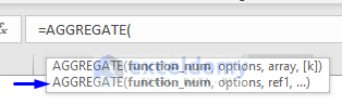
Syntax with Array Formula

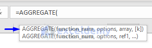
=AGGREGATE(function_num, options, array, [k])

• Arguments Description

Arguments in the Reference form,

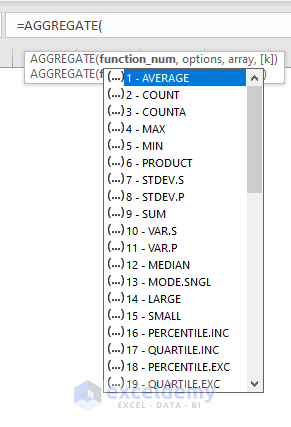function_num = Required, operations to perform. There are 19 functions are available to perform with the AGGREGATE function. Each function is defined by individual numbers. (see the table below)

options = Required, values to ignore. There are 7 values each representing the option to ignore while performing the operations with the functions defined.

ref1 = Required, the first numeric argument for functions to perform the operation. It could be one single value, array value, cell reference etc.

ref2 = Optional, it could be numeric values from 2 to 253

Arguments in the Array Formula,

function_num = (as discussed above)

options = (as discussed above)

array = Required, range of numbers or cell references based on that the functions will perform.

[k] = Optional, this argument is needed only when performing with the function number from 14 to 19 (see the function_num table).

Return Value

Return values based on the function specified.

In this section, you will learn how to use the AGGREGATE function in Excel with 13 effective examples.

1. Using the AGGREGATE Function in Excel to Calculate the AVERAGE

Let’s learn how to calculate the AVERAGE (statistical mean) of values with the AGGREGATE function. See the following example.

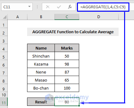
Here we got the AVERAGE result by running an AGGREGATE function. Look closely inside the parentheses of the function.

Here,

1 = function number, means the AVERAGE function

4 = option, means we will ignore nothing

C5:C9 = cell references that have the values to calculate the AVERAGE

2. Getting the Total COUNT of Values with the AGGREGATE Function

With the help of the AGGREGATE function, you can perform the COUNT function too. The COUNT function counts how many values are present in a defined range.

Look at the following example, there are 5 values in the Marks column, as a result, we got 5 as our result by performing an AGGREGATE function.

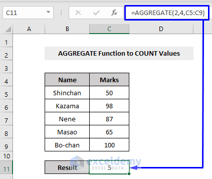
Here,

2 = function number, means the COUNT function

4 = option, means we will ignore nothing

C5:C9 = cell references that have the values to COUNT values

Similarly, you can perform the COUNTA function that counts values that hold both numeric and text values with the AGGREGATE function.

See the following example where the Marks column consisted of numbers and texts.

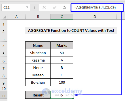
And by performing the COUNTA function inside the AGGREGATE function, we extracted the result, 5.

Here,

3 = function number, means the COUNTA function

4 = option, means we will ignore nothing

C5:C9 = cell references that have the values to count values with texts

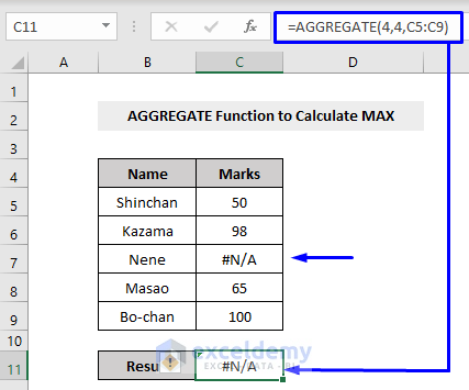
3. Extracting Maximum or Minimum Values with AGGREGATE Function in Excel

Okay, now you have got the hang of the idea of the AGGREGATE function. Now let’s try the function with different options.

In this section, we will find the Maximum and Minimum values among a range that has error values, hidden rows etc.

Look at the following picture. Here we will run the MAX function with the help of the AGGREGATE function to get the maximum value from the defined range.

If you are following this article from the beginning then you already know how to do that, just pass the function number of MAX function as the parameter of the AGGREGATE function. But to make this a bit tricky, we added a #N/A error in our dataset. So when we run the AGGREGATE function now, we will get errors.

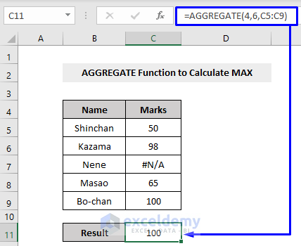
So to calculate MAX from a range consisting of error values, we have to set the options parameter as,

6 = means, we will ignore error values

After defining the parameter to ignore error values, now if we execute the MAX with the AGGREGATE function, we will still get our desired result even if we have error values lying in the dataset. (see the following picture)

To extract the minimum value from a dataset that has hidden rows, we have to set the parameter as,

5 = means, we will ignore hidden rows

It will produce the result based on the MIN function ignoring the value concealed in the hidden rows.

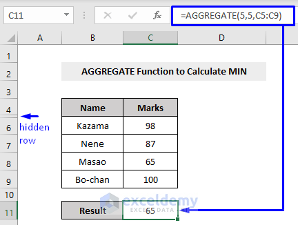
We had a minimum value, 50, in the 5th row. But as the row is hidden so our AGGREGATE function returns the next minimum value, 65.

Read More: How to Use AGGREGATE to Achieve MAX IF Behavior in Excel

4. Calculating SUM with the AGGREGATE Function

We all know how the SUM function works – adds all the values and returns the summation. But this time we will execute the SUM function with error values and hidden rows in it. And to do that with the AGGREGATE function, we have to set the options parameter 7 this time.

Consider the following example.

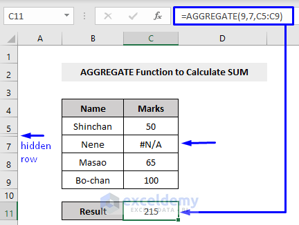
Here,

9 = function number, means the SUM function

7 = option, means we will ignore hidden rows and error values

C5:C9 = cell references that have the values to SUM the values

5. Using AGGREGATE Function in Excel to Measure the PRODUCT of Values

To multiply all the values of a defined range, you can utilize the PRODUCT function. The PRODUCT function returns the multiplicated result of all the values that you provide.

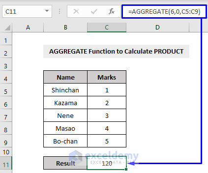
Here,

6 = function number, means the PRODUCT function

0 = option, as we are performing a generic PRODUCT function so we will ignore nested SUBTOTAL and AGGREGATE functions

C5:C9 = cell references that have the values to calculate the PRODUCT of the values

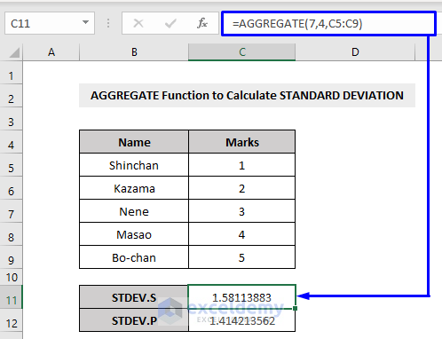
6. Excel’s AGGREGATE Function to Measure the Standard Deviation

Excel’s STDEV function is a statistical function, which refers to the Standard Deviation for a sample dataset.

The equation,

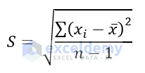
Here,

xi = takes on each value in the dataset

x¯ = average (statistical mean) of the dataset

n = number of values

With the AGGREGATE function, you can calculate the Standard Deviation for a sample dataset with the STDEV.S function (function number 7).

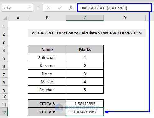
And to calculate the Standard Deviation for a whole population you can use the STDEV.P function (function number 8).

Read More: Combining AGGREGATE with IF Function in Excel

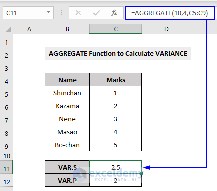
7. Applying the AGGREGATE Function in Excel to Calculate the VARIANCE

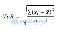
VAR function is another statistical function in Excel, which estimates the variance of a sample dataset.

The equation,

Here,

xi = takes on each value in the dataset

x¯ = average (statistical mean) of the dataset

n = number of values

To calculate the VARIANCE of a sample dataset with the AGGREGATE function, you have to use the VAR.S function, which is function number 10.

And to calculate the VARIANCE of an entire population, you have to use the VAR.P function, which is function number 11 in Excel.

8. Calculating MEDIAN Value with Excel AGGREGATE Function

The MEDIAN function in Excel returns the middle number of the set of data.

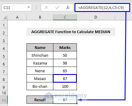
See the above example, there are 5 numbers, 50, 65, 87, 98, 100 – among which 87 is the middle number. So after performing the MEDIAN function with the help of AGGREGATE, we got the desired output, 87, in our result cell.

9. Applying the AGGREGATE Function to Measure the MODE in Excel

Excel’s MODE.SNGL function returns the most frequently occurred value within a range. This is also a statistical function in Excel.

Consider the following example, where 98 occurs 2 times, while the rest of the numbers occur only once.

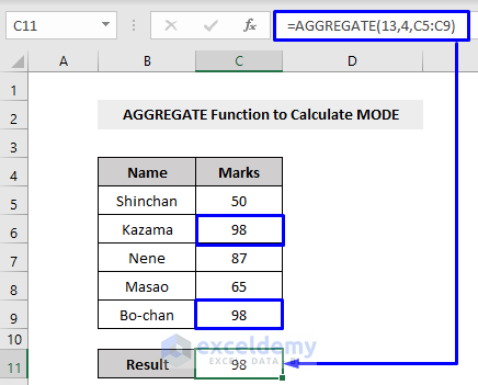
So by running the MODE function inside AGGREGATE throws the number 98 in our result cell.

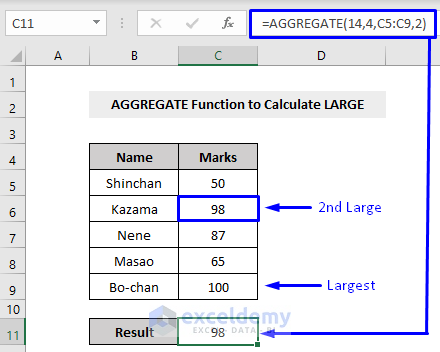
10. Calculating the LARGE Value with Excel’s AGGREGATE Function

The LARGE function returns the largest number among a given dataset. It holds function number 14, so that means when performing this function with the AGGREGATE, we need to insert the [k] as the fourth parameter.

Look at the following picture to understand more.

Here,

14 = function number, means the LARGE function

4 = option, means we will ignore nothing

C5:C9 = cell references that have the values to extract the result

2 = 2nd largest value (if you want to get the largest value within a dataset then write 1, if you want to get the 3rd largest value then write 3 and so on)

The largest value in our dataset is 100. But as we put 2 in the k-th argument, that means we wanted to have the 2nd largest value among our dataset. 98 is the 2nd largest so we got 98 as our output.

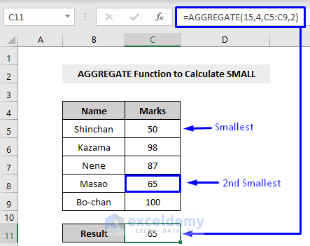
11. Measuring the SMALL Value with the AGGREGATE Function

Excel’s SMALL function returns the smallest number among a given dataset. It holds function number 15, so as discussed before when performing this function with the AGGREGATE, we need to insert the [k] as the fourth parameter.

Look at the following picture to understand more.

Here,

15 = function number, means the SMALL function

4 = option, means we will ignore nothing

C5:C9 = cell references that have the values to extract the result

2 = 2nd smallest value (if you want to get the smallest value within a dataset then write 1, if you want to get the 3rd smallest value then write 3 and so on)

The smallest value in our dataset is 50. But as we put 2 in the k-th argument, that means we wanted to have the 2nd smallest value among our dataset. As 65 is the 2nd smallest so we got 65 as our output.

12. Using the AGGREGATE Function to Measure the PERCENTILE in Excel

The PERCENTILE function in Excel calculates the k-th percentile for a set of data. A percentile is a value below which a given percentage of values in a data set fall.

The value of k can be decimal or percentage-wise. Meaning, for the 10th percentile, the value should be entered as 0.1 or 10%.

For instance, a percentile calculated with 0.2 as k means 20% of values are less than or equal to the calculated result, a percentile of k = 0.5 means 50% of the values are less than or equal to the calculated result.

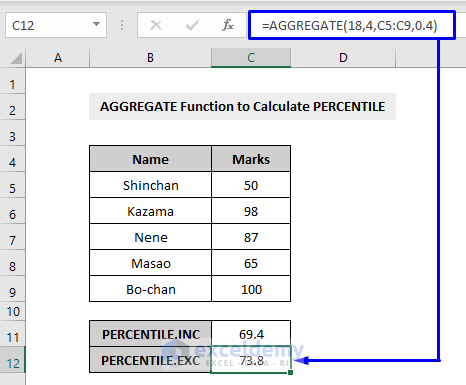
The AGGREGATE function holds the PERCENTILE.INC (function number 16) and the PERCENTILE.EXC (function number 18) to calculate the percentile value of a given dataset.

The PERCENTILE.INC returns the inclusive k-th percentile between 0 and 1.

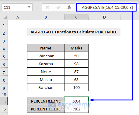
The PERCENTILE.EXC returns the exclusive k-th percentile between 0 and 1.

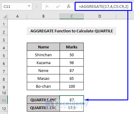
13. Calculating the QUARTILE with the AGGREGATE Function in Excel

Excel’s QUARTILE function returns the quarter part (each of four equal groups) of a whole set of data.

The QUARTILE function accepts five values,

0 = Minimum value

1 = First quartile, 25th percentile

2 = Second quartile, 50th percentile

3 = Third quartile, 75th percentile

4 = Maximum value

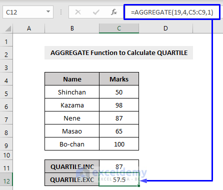
The AGGREGATE function works with QUARTILE.INC (function number 17) and QUARTILE.EXC (function number 19) function to produce the quartile results.

The QUARTILE.INC function calculates based on a percentile range of 0 to 1 inclusive.

The QUARTILE.EXC function calculates based on a percentile range of 0 to 1 exclusive.

Download Practice Workbook

You can download the free practice Excel workbook from here.

Conclusion

This article explained everything in detail about the AGGREGATE function in Excel. I hope this article has been very beneficial to you. Feel free to ask if you have any questions regarding the topic.

Excel AGGREGATE Function: Knowledge Hub

<< Go Back to Excel Functions | Learn Excel