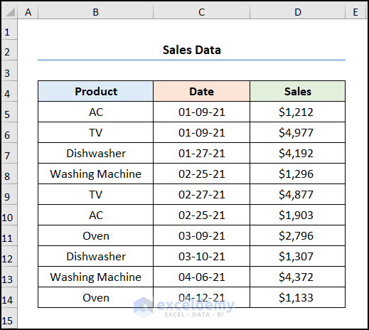
The sample dataset showcases Sales Data: Product names, sales Date, and Sales in USD.
Method 1 – Utilizing COUNTIF Function with Greater Than and Less Than Criteria
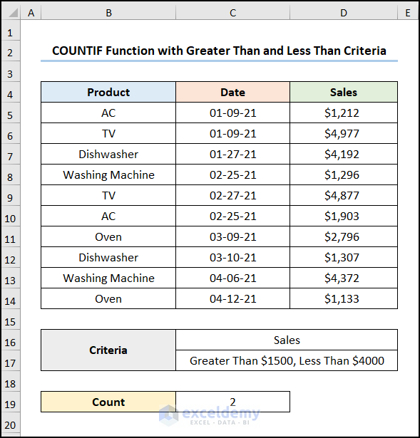
To find Sales values between $1500 and $4000.
Steps:
- Select C19 and enter the following formula.
=COUNTIF(D5:D14,">1500")-COUNTIF(D5:D14,">=4000")
Formula Breakdown:
- COUNTIF(D5:D14,”>1500”) → counts the number of cells within a range that meet the given condition. D5:D14 is the range argument that refers to Sales.”>1500” is the criteria argument that returns the count of the matched values.
- Output → 6
- COUNTIF(D5:D14,”>=4000”) → D5:D14 is the range argument that refers to Sales. ”>=4000” is the criteria argument that returns the count of the matched values.
- Output → 4
- COUNTIF(D5:D14,”>1500″)-COUNTIF(D5:D14,”>=4000″) → becomes
- 6-4 → 2
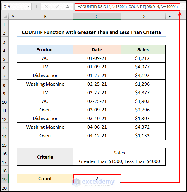
This is the output.
Read More: How to Aggregate Data in Excel
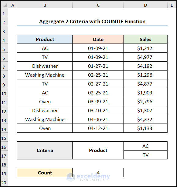
Method 2 – Aggregate 2 Criteria with the COUNTIF Function
To count the occurrences of AC and TV in the dataset:
Steps:
- Select C19 and enter the following formula.
=COUNTIF(B5:B14,D16)+COUNTIF(B5:B14,D17)
Formula Breakdown:
- COUNTIF(B5:B14,D16) → counts the number of cells within a range that meet the given condition. B5:B14 is the range argument that refers to Sales. D16 is the criteria argument that returns the count of the matched values.
- Output → 2
- COUNTIF(B5:B14,D17) → D5:D14 represents the range argument that refers to Sales. D17 is the criteria argument that returns the count of the matched values.
- Output → 2
- COUNTIF(B5:B14,D16)+COUNTIF(B5:B14,D17) → becomes
- 2+2 → 4
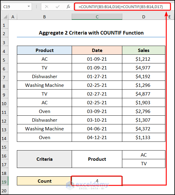
This is the output.
Read More: How to Use Excel AGGREGATE Function with Multiple Criteria
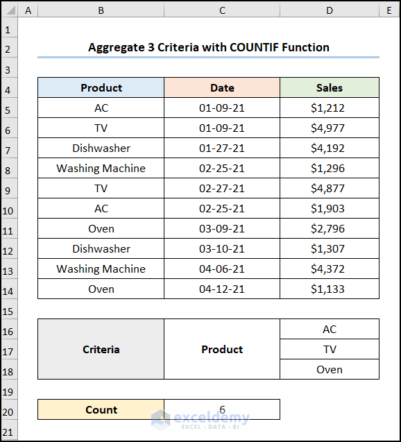
Method 3 – Aggregate 3 Criteria with the COUNTIF Function
Determine the occurrences of AC, TV, and Oven:
Steps:
- Select C19 and enter the following formula.
=COUNTIF(B5:B14,D16)+COUNTIF(B5:B14,D17)+COUNTIF(B5:B14,D18)
D16, D17, and D18 are the Criteria AC, TV, and Oven.
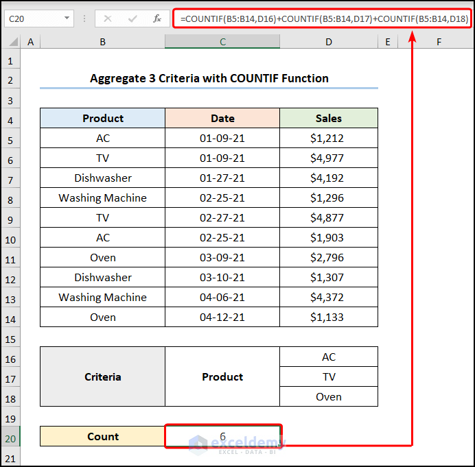
This is the output.
Read More: How to Use Conditional AGGREGATE Function in Excel
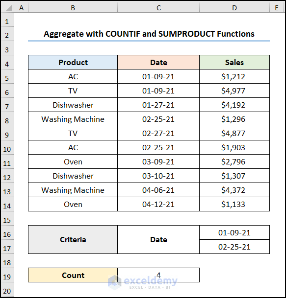
Method 4 – Using the COUNTIF and the SUMPRODUCT Functions
Find specified dates in the dataset.
Steps:
- Select C19 and enter the following formula.
=SUMPRODUCT(COUNTIF(C5:C14,{"01-9-21","02-25-21"}))
Formula Breakdown:
- COUNTIF(C5:C14,{“01-9-21″,”02-25-21”}) → C5:C14 is the range argument that refers to Dates. {“01-9-21″,”02-25-21”} is the criteria argument that returns the count of the matched values.
- Output → {2, 2}
- SUMPRODUCT(COUNTIF(C5:C14,{“01-9-21″,”02-25-21”})) → becomes
- SUMPRODUCT({2, 2}) → returns the sum of the products of the corresponding ranges or arrays. Here, {2, 2} is the array1 argument which is added to return the number of occurrences of the specified criteria.
- Output → 4
Note: Press CTRL+SHIFT+ENTER instead of ENTER when using Excel versions, other than Microsoft Excel 365.
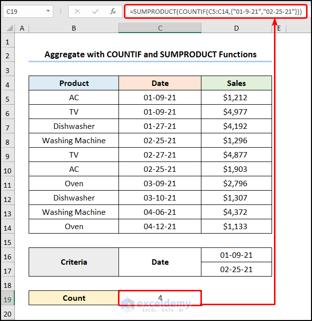
This is the output.
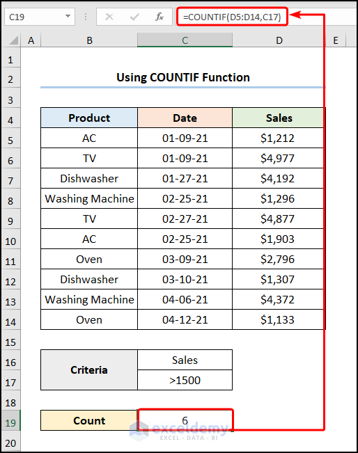
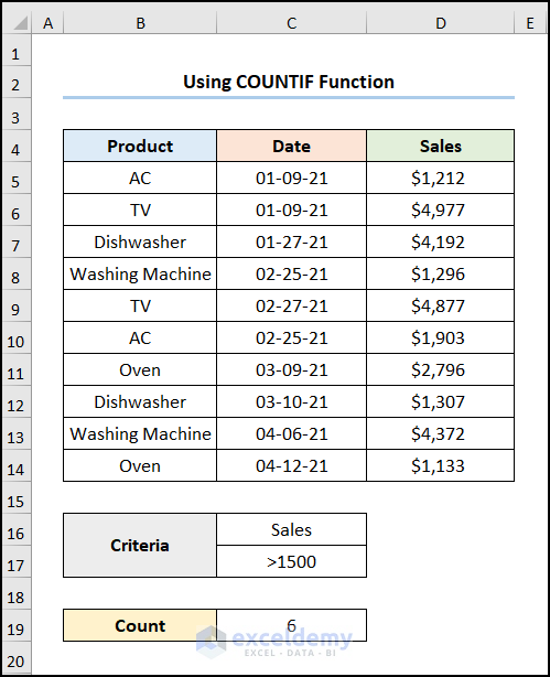
Using the COUNTIF Function to Aggregate Counting Values in Excel
To count Sales greater than $1500:
Steps:
- Select C19 >> enter the formula below.
=COUNTIF(D5:D14,C17)
Formula Breakdown:
- COUNTIF(D5:D14,C17) → counts the number of cells within a range that meet the given condition. D5:D14 represents the range argument that refers to Sales. C17 is the criteria argument that returns the count of the matched values.
- Output → 6
This is the output.
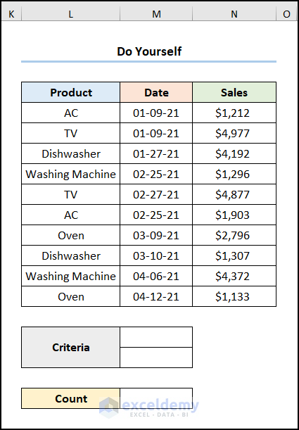
Practice Section
Practice here.
Download Practice Workbook
Download the practice workbook.
Related Articles
- AGGREGATE vs SUBTOTAL in Excel
- AGGREGATE Formula for Adding Serial Number in Excel
- Combining AGGREGATE with IF Function in Excel
- How to Combine INDEX and AGGREGATE Functions in Excel
<< Go Back to Excel AGGREGATE Function | Excel Functions | Learn Excel
Get FREE Advanced Excel Exercises with Solutions!
