If you are searching for some special tricks to use the Excel AGGREGATE function with multiple criteria then you have landed in the right place. There are some tricks in using the AGGREGATE function with multiple criteria in Excel. This article will show you each and every step with proper illustrations so, you can easily apply them for your purpose. Let’s get into the central part of the article.
An Overview of Excel AGGREGATE Function
The AGGREGATE function is used on different functions like AVERAGE, COUNT, MAX, MIN, SUM, PRODUCT etc. with the option to ignore hidden rows and error values to get certain results.
Syntax of AGGREGATE Function:
- Syntax with References
=AGGREGATE(function_num, options, ref1, ref2, …)
- Syntax with Array Formula
=AGGREGATE(function_num, options, array, [k])
Descriptions of the Arguments:
- Function_Num = It is a required Argument and defines which task to do. There are 19 functions available to perform with the AGGREGATE function. Individual numbers define each function. (see the table below)
| Function Name | Function Number |
|---|---|
| AVERAGE | 1 |
| COUNT | 2 |
| COUNTA | 3 |
| MAX | 4 |
| MIN | 5 |
| PRODUCT | 6 |
| STDEV.S | 7 |
| STDEV.P | 8 |
| SUM | 9 |
| VAR.S | 10 |
| VAR.P | 11 |
| MEDIAN | 12 |
| MODE.SNGL | 13 |
| LARGE | 14 |
| SMALL | 15 |
| PERCENTILE.INC | 16 |
| QUARTILE.INC | 17 |
| PERCENTILE.EXC | 18 |
| QUARTILE.EXC | 19 |
- Options = Required, values to ignore. There are 7 values each representing the option to ignore while performing the operations with the functions defined.
| Option Number | Option Name |
|---|---|
| 0 or omitted | omit nested AGGREGATE and SUBTOTAL functions |
| 1 | omit hidden rows, nested SUBTOTAL, and AGGREGATE functions |
| 2 | leave out error values, nested SUBTOTAL, and AGGREGATE functions |
| 3 | omit hidden rows, error values, nested SUBTOTAL, and AGGREGATE functions |
| 4 | leave out nothing |
| 5 | leave out hidden rows |
| 6 | omit error values |
| 7 | Ignore hidden rows and error values |
- Ref1 = Required, the first numeric argument for functions to perform the operation. It could be one single value, array value, cell reference, etc.
- Ref2 = Optional, it could be numeric values from 2 to 253.
- Array = Required for Array Formula. It is the range of numbers or cell references based on the performance of the functions.
- [k] = Optional in Array Formula, this argument is needed only when performing with the function number from 14 to 19.
How to Use Excel AGGREGATE Function with Multiple Criteria: 3 Examples
In this section, I will show you the quick and easy steps to use the Excel AGGREGATE function with multiple criteria on the Windows operating system. You will find detailed explanations with clear illustrations of each thing in this article. I have used the Microsoft 365 version here. But you can use any other versions as of your availability. If anything in this article doesn’t work in your version then leave us a comment.
Example 1: Find the nth Smallest Value Using AGGREGATE Function with Multiple Criteria
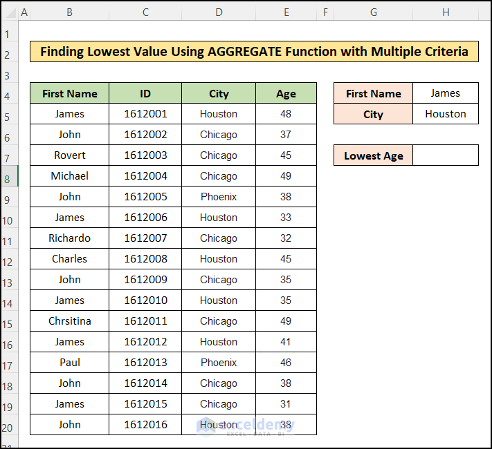
In this example, I will show you how you can use the AGGREGATE function to find the lowest or nth lowest value meeting multiple criteria. I have a dataset where I have columns containing persons’ first names, IDs, Names of Cities where they live, and Ages. So, I want to get the values of the lowest age among the persons whose name is “James” and who live in Houston city.
📌 Steps:
- For this, first, assign 2 cells to get input of the Name and City. I have assigned cell H4 for First Name and H5 for City.
- Then, assign a cell to get the lowest age following the previously mentioned
- Then, insert the following formula into cell H7:
=AGGREGATE(16,6,E5:E20/((H4=B5:B20)*(H5=D5:D20)),1)🔎 Formula Breakdown:
- Function_num = 16: It is used to find the smallest value of the selected range.
- Options = 6: It commands to ignore the error values.
- Array = E5:E20/((H4=B5:B20)*(H5=D5:D20)): It defines the criteria for the array E5:E20. The first criterion is to match the cell H4 in range B5:B20 and the second criterion is to match cell H5 in range D5:D20.
- [k] = 1: Here, 1 is used to get the lowest value in the range meeting the criteria and you can use 2,3, or n to find the 2nd, 3rd, or nth smallest values of the specified range.
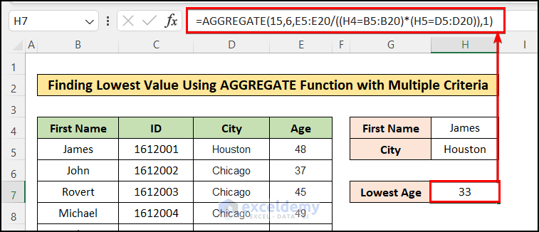
- Thus, you have got the lowest age of people named “James” and living in “Houston” city using the AGGREGATE
- Also, you can get the 2nd, 3rd, or nth smallest value by assigning the fourth argument, k accordingly.
✅ Note:
Multiple criteria in the array of the AGGREGATE function are only applicable for function numbers 14 to 19.
Read More: How to Aggregate Data in Excel
Example 2: Find the nth largest Value Using AGGREGATE Function with Multiple Criteria
Similarly, you can use the AGGREGATE function to get the Highest or the largest value of the range that meets the criteria. For this, you have to specify the Function_Num as 14 which works to find the largest value. Insert the following formula into cell H7 to find the largest value:
=AGGREGATE(14,6,E5:E20/((H4=B5:B20)*(H5=D5:D20)),1)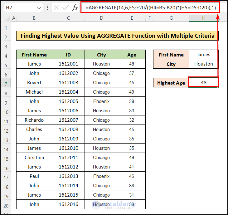
Example 3: Find Percentile Using AGGREGATE Function with Multiple Criteria
In addition, the AGGREGATE Percentile in Excel calculates the k-th percentile for a set of data. A percentile is a value below which a given percentage of values in a data set fall.
For this, you have to specify the Function_Num as 16 which works to find the Percentile. The value of k can be decimal or percentage-wise. This means, that for the 10th percentile, the value should be entered as 0.1 or 10%. Insert the following formula into cell H7 to find the Percentile:
=AGGREGATE(16,6,E5:E20/((H4=B5:B20)*(H5=D5:D20)),0.1)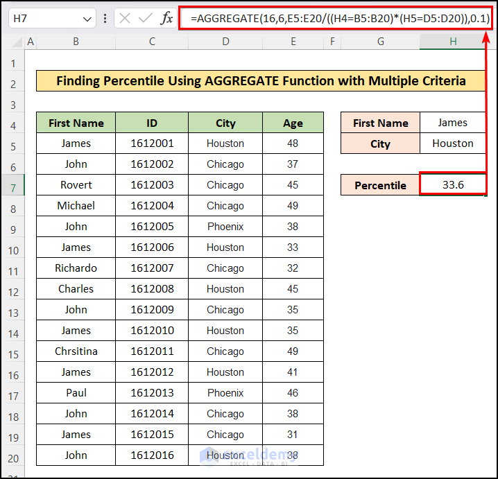
Similarly, you can calculate Quartile and Percentile values using the corresponding Function Number mentioned above.
Read More: How to Use Conditional AGGREGATE Function in Excel
How to Use INDEX-MATCH with Excel AGGREGATE Function for Multiple Criteria
In this case, I will show you how to combine INDEX and AGGREGATE functions in Excel to calculate the total sum of given data in a certain period. We will do this by the following steps.
📌 Steps:
- First, arrange a dataset like the following image.
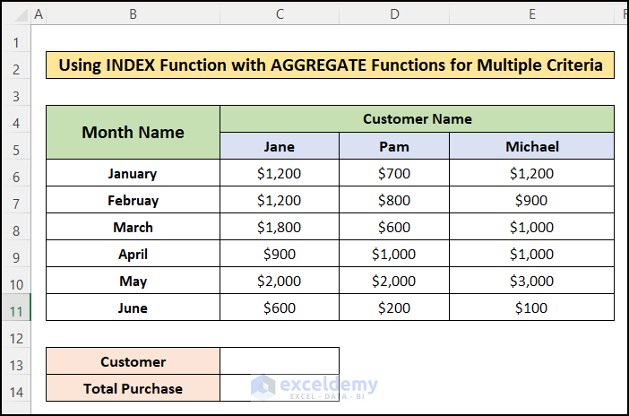
- Next, in the C13 cell insert the name of the desired customer similar to the following image.
- After that, in the C14 cell insert the following formula.
=AGGREGATE(9,0,INDEX(C6:E11,,MATCH(C13,C5:E5,0)))🔎 Formula Breakdown:
- MATCH(C13, C5:E5,0) = 3: First, the MATCH function works to find the matches of cell C13 in the range C5:E5.
- INDEX(C6:E11, ,MATCH(C13, C5:E5,0)) = {1200;900;1000;1000;3000;100}: Then, the INDEX function works to return the cells of the column specified by the Match function.
- AGGREGATE(9,0,INDEX(C6:E11,,MATCH(C13,C5:E5,0)))): Finally, the AGGREGATE function sums the list made by the INDEX function.
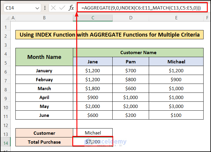
- Finally, you will get the desired result similar to the following image.
Download Practice Workbook
You can download the practice workbook from here:
Conclusion
In this article, you have found how to use the Excel AGGREGATE function with multiple criteria. I hope you found this article helpful. Please, drop comments, suggestions, or queries if you have any in the comment section below.
Related Articles
- How to Use AGGREGATE to Achieve MAX IF Behavior in Excel
- AGGREGATE vs SUBTOTAL in Excel
- How to Aggregate COUNTIF in Excel
- Combining AGGREGATE with IF Function in Excel
- AGGREGATE Formula for Adding Serial Number in Excel
<< Go Back to Excel AGGREGATE Function | Excel Functions | Learn Excel
Get FREE Advanced Excel Exercises with Solutions!
