How to Use AGGREGATE to Achieve MAX IF Behavior in Excel

Microsoft Excel is a powerful software. There are many default Excel Functions that we can use to create formulas. Many educational institutions and business companies use Excel files to store valuable data. Sometimes, we need to find the maximum value based on certain conditions. We can do that by combining the MAX and IF functions. Moreover, the MAXIFS function can also do the job. However, the AGGREGATE function can perform a similar task with some additional benefits like ignoring error values. This article will show you 3 ideal examples of using AGGREGATE to achieve MAX IF behavior in Excel.

How to Use AGGREGATE to Achieve MAX IF Behavior in Excel: 3 Examples

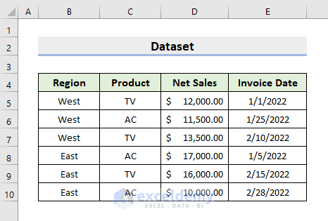
The AGGREGATE function can carry out various operations depending on the Function Number that we’ll input in the argument. Then, we can decide on what to ignore by choosing the Option Number. Subsequently, we have to select the Array on which we’ll perform the operations. Here, we’ll show how you can use this function to achieve the MAX IF behavior. To illustrate, we’ll use a sample dataset as an example. For instance, the following dataset contains Region, Product, Net Sales, & Invoice Date. This article will show the process to extract the maximum sales of a product from a particular region.

1. Use AGGREGATE Function for MAX IF to Find Last Date in Excel

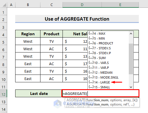
In our first example, we’ll determine the last invoice date for the product TV. The last date will have the maximum value in terms of numbers. In this regard, we’ll input 14 as the function number. 14 is for the LARGE function. If you select function number 4 which is MAX, you’ll get an error. Because it can’t calculate based on conditions. Therefore, follow the steps below to perform the task.

STEPS:

First, select cell D12.
Then, type the formula:

=AGGREGATE(

As a result, you’ll see the function numbers along with the function names.
Double-click the LARGE function.

Consequently, choose the option number that suits your requirements.
In this example, we choose 6 (Ignore error values).

Now, type the array:

(E5:E10)/(C5:C10=C5)

Finally, the formula is:

=AGGREGATE(14,6,(E5:E10)/(C5:C10=C5),1)

Next, press Enter to get the output.
Thus, you’ll get the last invoice date for TV.

NOTE: In the array section, E5:E10 is the Net Sales range. And C5:C10=C5 looks for the product TV. 1 is for the 1st largest number.

2. Determine Maximum Based on Criteria with Excel AGGREGATE Function

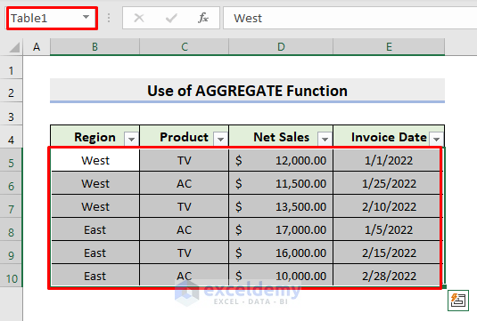
Now, we’ll show how you can get the maximum Net Sales of TV. However, instead of using cell range in the array argument, we’ll input table reference. You can easily create a table by pressing the Ctrl and T keys together after selecting the desired range. In this example, the condition is TV. So, learn the following steps to determine maximum sales based on single criteria with the Excel AGGREGATE function. We’ll use 14 as the function number and 6 as the option number for this example.

STEPS:

Firstly, we create a table (Table1) by selecting the range B4:E10.
See the picture below where we have the table.

After that, input the formula:

=AGGREGATE(14,6,Table1[

Hence, the table headers will pop out.
Choose Net Sales.

Afterward, type /Table1[ and table headers will appear again.
There, select Product.

Lastly, the whole formula is:

=AGGREGATE(14,6,Table1[Net Sales]/(Table1[Product]="TV"),1)

Next, press Enter.
Consequently, you’ll get an accurate result.

NOTE: Table1[Product]=”TV” looks for TV in the Product range. And 1 is for the 1st maximum value.

3. Insert AGGREGATE to Achieve Maximum Based on Double Criteria

However, we may face real-life problems where we have to find out the maximum value from a range based on multiple conditions. In our last example, we’ll demonstrate how you can do that with the AGGREGATE function. The conditions are West and TV as the Region and the Product respectively. Hence, follow the process below.

STEPS:

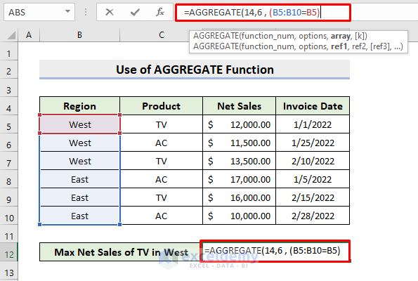
First of all, click cell D12.
Then, type the formula:

=AGGREGATE(14,6,(B5:B10=B5)

Here, B5:B10=B5 matches the first condition which is West as Region.

Next, type *(C5:C10=C5), and the formula becomes:

=AGGREGATE(14,6,(B5:B10=B5)*(C5:C10=C5)

Subsequently, this part looks for the product TV.

Finally, put *D5:D10,1 and the complete formula is:

=AGGREGATE(14,6,(B5:B10=B5)*(C5:C10=C5)*D5:D10,1)

Press Enter.
In this way, it’ll return the maximum value based on double criteria.

NOTE: D5:D10 is the Net Sales range from which we’ll extract the maximum value. 1 is for the 1st largest value.

Download Practice Workbook

Download the following workbook to practice by yourself.

Use AGGREGATE to Achieve MAX IF.xlsx

Conclusion

Henceforth, you will be able to use AGGREGATE to achieve MAX IF behavior in Excel following the above-described examples. Keep using them and let us know if you have more ways to do the task. Don’t forget to drop comments, suggestions, or queries if you have any in the comment section below.