AGGREGATE Formula for Adding Serial Number in Excel

While working with a large dataset, you may find it very boring and monotonous to write the serial number manually. The Autofill/Fill Handle is a very familiar way to solve this problem. But if you need to omit a row in the dataset, this method becomes faulty as it shows errors. Excel shines here by providing us with some extraordinary functions e.g. AGGREGATE function to make serial numbers automatically. In this article, we’re going to show you how to use the AGGREGATE formula for generating serial number in Excel. We’ll also discuss some other functions to make serial numbers in Excel. Let’s get started.

AGGREGATE Formula for Adding Serial Number in Excel: 3 Methods

You can use the AGGREGATE function for serial numbers in Excel. You have to give both the COUNT and COUNTA functions as arguments and create serial numbers. We can also use the SUBTOTAL function instead of the AGGREGATE formula for serial numbers in Excel. We have taken a dataset of Student’s CGPA of a university. Now, we will show you the way to use the formula for adding serial numbers in Excel.

Not to mention, we have used Microsoft 365 version. You may use any other version at your convenience

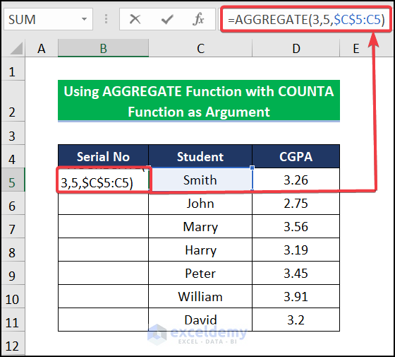
1. Using AGGREGATE Function with COUNTA Function as Argument

You may use the AGGREGATE function where the COUNTA function will be an argument. By applying this function, you can easily find the serial number in your dataset. It will reduce your difficulties and save time. Follow the below steps to do that.

📌 Steps:

• First of all, go to cell B5 and write down the formula.

Here,

C5= The cell from where the counting starts.

• Subsequently, press ENTER and drag down the Fill Handle tool for other cells.

• Finally, you will get the serial numbers for your worksheet.

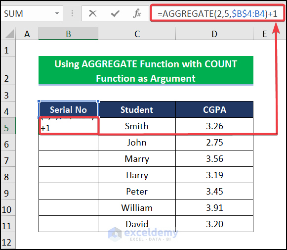
2. Utilizing AGGREGATE Function with COUNT Function as Argument

We also use the AGGREGATE function with the COUNT function as an argument to make serial numbers in Excel. Basically, it refreshes automatically when you delete a row or any cell. To get a proper visualization, please follow the steps we have discussed below.

📌 Steps:

• Initially, select cell B5 and write up the formula.

Here,

The AGGREGATE(2,5,$B$4:B4)+1 syntax will take the COUNT function as function_num and it takes 5 as the reference to Ignore hidden rows. Then it will take the option array of $B$4:B4. We enter a +1 for completing the formula immediately after cell B4.

• Press ENTER and drag down the formula for other cells.

Eventually, you will get the result.

Read More: How to Aggregate Data in Excel

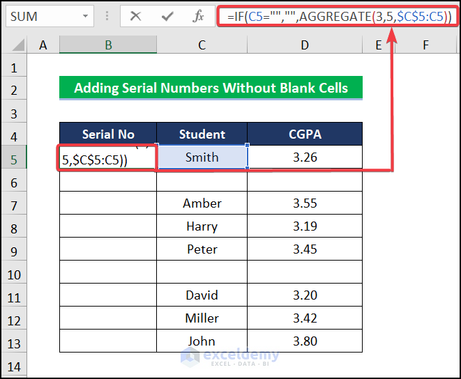
3. Generating Serial Number Ignoring Blank Cells

Sometimes, your dataset may contain blank cells where you don’t need to apply for the serial number. But if you use the Fill Handle tool for creating serial numbers, then it will cover the blank cell as well as the number. To avoid this consequence, we will use the IF function nested with the AGGREGATE function for serial numbers in blank cells.

📌 Steps:

• In the very beginning, enter the formula in cell B5.

• Press ENTER and continue this formula for other cells using Fill Handle.
• Finally, you will get the serial number excluding blank cells.

Read More: Combining AGGREGATE with IF Function in Excel

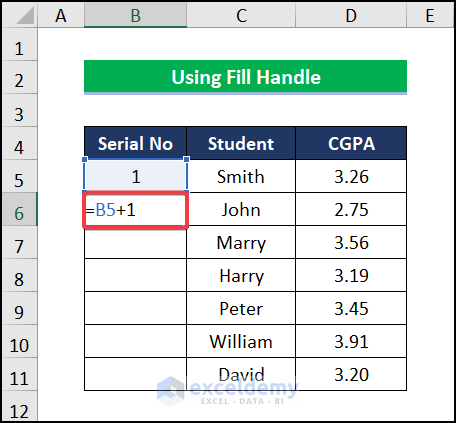
Using Shortcut for Adding Serial Number in Excel

The easiest way to enter the serial number in your sheet is to apply the AutoFill shortcut. Though it is a simple way, it becomes difficult for the customer to handle in the case of a blank cell or in the operation of deleting the rows. Putting this aside, we show you the steps to follow for using this method.

📌 Steps:

• First of all, give the serial number 1 in your first cell and then go to the next cell B6 and simply enter

• Press ENTER.
• Drag down the AutoFill feature or press CTRL + D as a keyboard shortcut to copy the same formula to other cells.

• Lastly, you will get the results.

Read More: How to Use Excel AGGREGATE Function with Multiple Criteria

Using SUBTOTAL Formula as an Alternative to AGGREGATE Formula

The SUBTOTAL function is an alternative to the AGGREGATE function to create the serial numbers in your sheet. It also takes the COUNTA function as an argument. All you need to put the argument and select the cells where you want to give the serial numbers.

📌 Steps:

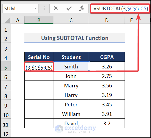
• Primarily, select B5 and write down the formula.

Here, the syntax SUBTOTAL(3,$C$5:C5) will take function_num i.e. 3 as the argument of the COUNTA function. Then select the first $C$5:C5 cell for the option array.

• Consequently, press ENTER and drag it down.
• Finally, you will get the serial numbers.

Read More: AGGREGATE vs SUBTOTAL in Excel

How to Auto Generate Serial Number Based on Another Column in Excel

You may give the serial numbers based on other columns. To do this, we will use the SEQUENCE and ROWS functions. It will create sequential serial numbers in your dataset. Follow the simple steps stated below.

📌 Steps:

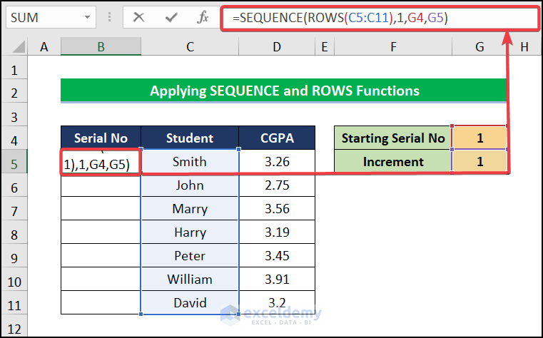
• Firstly, select cell B5 and insert the formula.

• Press ENTER.
• Finally, you will get the result.

Practice Section

We have provided a practice section on each sheet on the right side for your practice. Please do it by yourself.

Download Practice Workbook

Download the following practice workbook. It will help you to realize the topic more clearly.

Conclusion

That’s all about today’s session. These are some easy methods for using the AGGREGATE formula for adding the serial number in Excel. Please let us know in the comments section if you have any questions or suggestions. For a better understanding please download the practice sheet. Thanks for your patience in reading this article.

Related Articles

• How to Use Conditional AGGREGATE Function in Excel
• How to Combine INDEX and AGGREGATE Functions in Excel
• How to Use AGGREGATE to Achieve MAX IF Behavior in Excel
• How to Aggregate COUNTIF in Excel