How to Use Nested IF Function in Excel (7 Examples)

When a function is inserted inside another function, then it is called a nested function. In this article, we will learn how to use the nested IF function in Excel.

In general, the IF function allows a user to perform conditional calculations based on specific criteria. However, when you have multiple conditions to evaluate, you may need to use the nested IF function.

Introduction to Nested IF Function in Excel

The nested IF function in Excel is a logical function that allows you to perform tests with multiple conditions and return different values based on the results of those tests. It is called “nested” because one IF function is nested inside another IF function.

• Syntax of IF Function

• Argument

The syntax for a nested IF function is similar to that of a regular IF function. As the nested IF formula holds multiple IF functions, the general expression is like:

You can add more conditions according to your needs inside the formula.

How to Use Nested IF Function in Excel: 7 Suitable Examples

While performing multiple operations in Excel based on criteria, the nested IF function is frequently used to extract specific outputs. In this section, we will see 7 ideal examples of how to use the nested IF function in Excel. Later, we will also see some alternatives to the nested IF function.

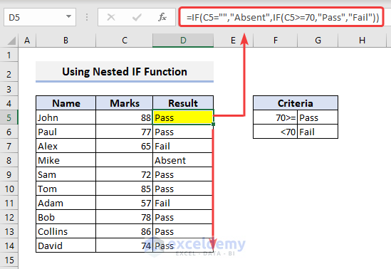
1. Use Nested IF Function to Find Multiple Results Based on Criteria

Let’s figure out a simple example to use the nested IF function in Excel. In this example, we will try to find the results of some students.  We have some students’ names in column B and the marks obtained by them in column C. Here, we are using three conditions.

• First, if a student gets 70 or higher, then he will pass.
• Second, if he gets less than 70, then he will fail.
• Third, if there is no mark, then, the student will be considered absent.

Insert the following formula in cell D5.

Read More: How to Create a Nested Formula in Excel

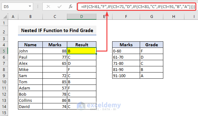
2. Find Grade Using Nested IF Function

In the second example, we will use the nested IF function in Excel to find the grades of some students. It is one of the most used examples to describe the nested IF function. For this example, we will use a dataset that contains the marks of some students. Here, the range of marks and corresponding grades are also given. We need to evaluate the grades of the students based on their obtained marks.

Apply the following formula in cell D5:

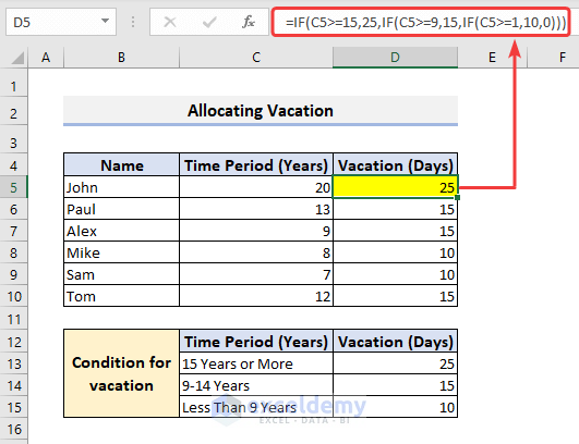
3. Apply Nested IF Function to Allocate Vacation Days

In the third example, we will try to allocate a Vacation period for employees of a company. To allocate a vacation period, we have introduced some conditions. If the employment period of an employee is 15 years or more, then he will have 25 vacation days. If it is between 9 to 14 years, then he will have 15 vacation days. And lastly, if the employment period is less than 9 years, then he will have 10 vacation days.

Apply the following formula in cell D5 to get the corresponding vacation days.

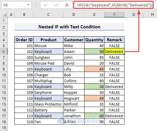
4. Use Nested IF Function with Text Condition

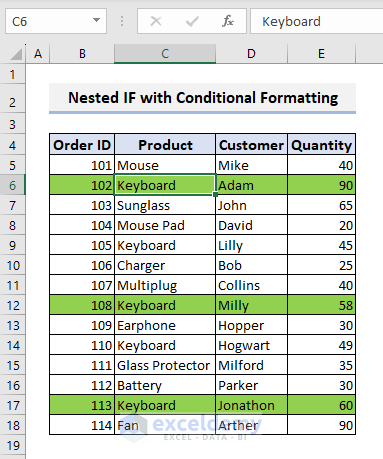
Previously we have used the nested IF with cell reference. In some cases, we may need to deal with conditions in text format. Consider the dataset stated below. We have a dataset of some customers who ordered different products of different quantities. For a specific condition, let’s say, if any customer orders more than 50 “Keyboard” at a single time, his order will be delivered. So, in that case. The text condition is “Keyboard”.

5. Insert Nested IF with Logical Operator

Usually, two types of logical operations are performed with the IF function: AND/OR.

5.1. Nested IF with OR Function

Here, we will see the application of the OR function with the nested IF function.

To explain the example, we will use a dataset that contains information about the sales amount for March & April. We will distribute the Sales Commission based on their sales amount.

Apply the following formula in cell E5.

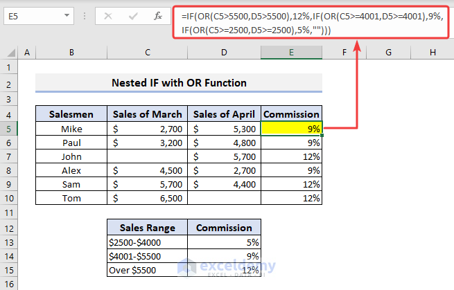
Note: The Number Format of the range E5:E10 must be set to Percentage. Otherwise, it will show 0.

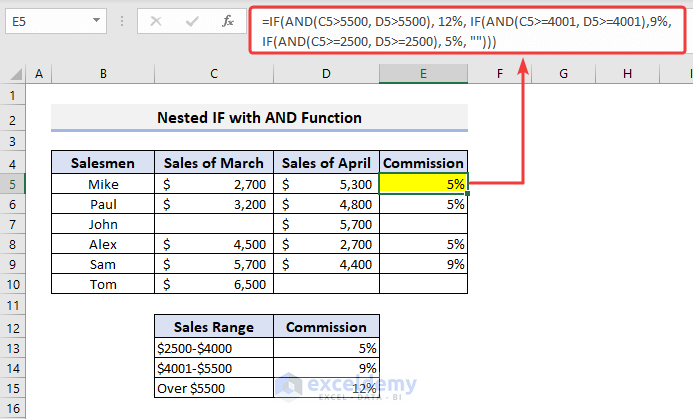
5.2. Nested IF with AND Function

Let’s apply the AND function with nested IF now. In that case, the formula will be:

Read More:How to Use Nested IF and SUM Formula in Excel

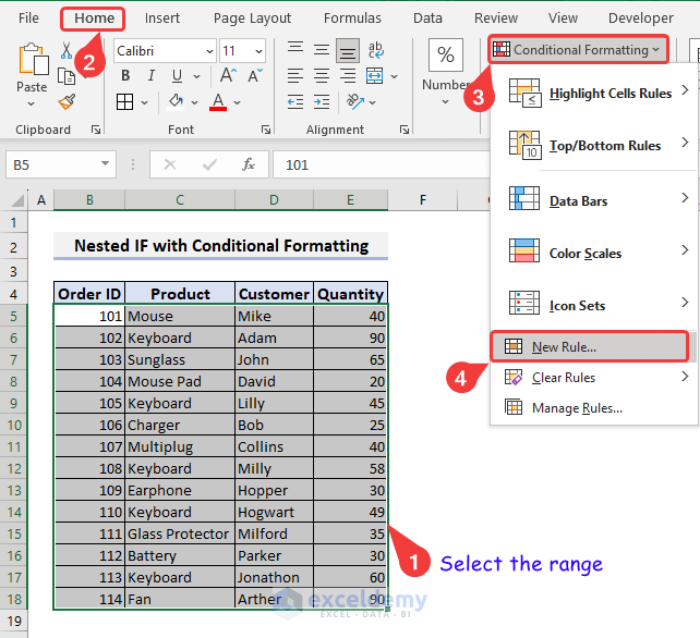
6. Apply Nested IF in Conditional Formatting

You can use the nested IF function to apply Conditional Formatting. Conditional formatting is used to highlight cells based on condition. For the dataset in the previous method, let’s highlight the row containing “Keyboard” over the quantity of “50”.

• Select the range of data >> go to Home tab >> click dropdown of Conditional Formatting >> select New Rule.

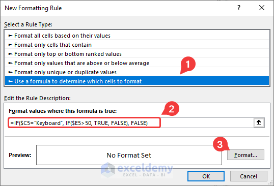
• The New Formatting Rule dialog box will appear.
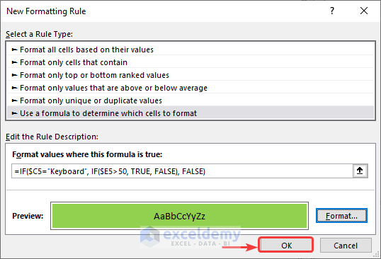
• Select “Use a formula to determine which cells to format” from the Select a Rule Type field.
• Use the formula below:

• Click Format.

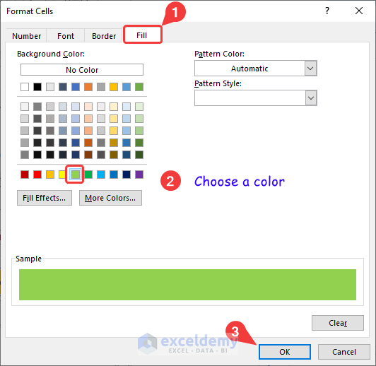
• From the Format Cells dialog box, go to Fill icon >> select a color >> click OK.

• Close the New Formatting Rule dialog box by clicking OK.

You will find that the rows containing “Keyboard” with a quantity of over “50” are highlighted.

7. Use TODAY Function with Nested IF Function to Determine Payment Status

In practical life, we need to determine the payment status often. Service-providing organizations need to keep a record of payments of their customers. In those cases, we can also use the TODAY function nested in the IF function.

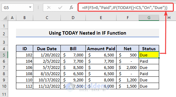
In the dataset below, we can see the Bills and Paid Amounts of some customers. Using this information, we will try to update the Status column.

So, apply the formula below in the first cell (i.e. G5) of the “Status” column

Alternative Approaches to Nested IF Function in Excel

It becomes difficult to implement the nested IF function if you have a lot of conditions. The formula may get bigger and any small mistake can lead to incorrect results. To avoid the difficulties, you can use the alternatives of the nested IF function in Excel. Here, we will discuss 5 alternatives. You can use them according to your needs.

1. Use VLOOKUP Function

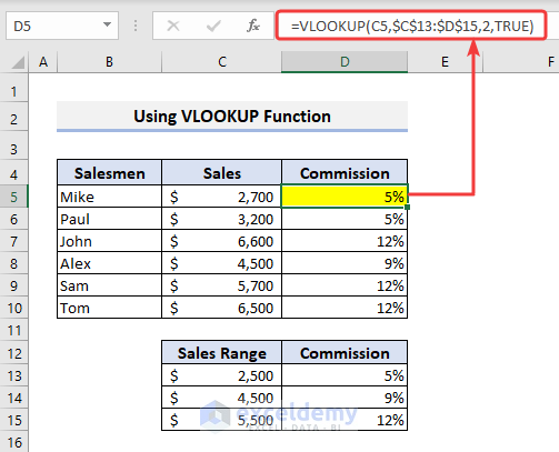
When you are using continuous ranges of numbers, then you can use the VLOOKUP function instead of the nested IF function. For this purpose, you need to have a reference table and create the formula with the approximate match. In our case, the Commission table is our reference table. In the dataset, we have a sales amount for each salesman and will try to allocate the commission.

Here, our formula will be:

Here, we have used the VLOOKUP function to look for the value of Cell C5 in the second column of the lookup table ranging from Cell C13 to D15. We need to apply the approximate match here, so we used TRUE in the last argument of the formula.

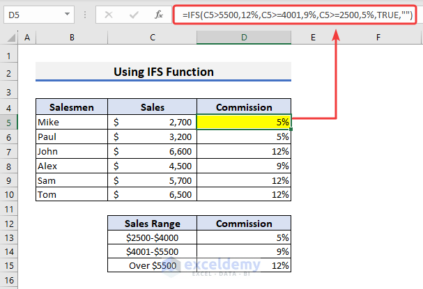
2. Apply IFS Function

The application of the IFS function makes the task of implementing multiple conditions very easy. For a similar dataset as above, our formula will be as below:

Here, Test 1 is to check whether Cell C5 is greater than 5500. If TRUE, then it will show 12 %. Otherwise, it will move to Test 2 and so on.

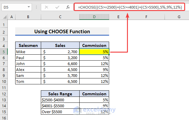
3. Insert CHOOSE Function

We can also use the CHOOSE function to check multiple conditions. The CHOOSE function returns a value from the list based on the index number of that value.

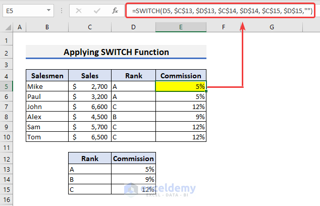
4. Apply SWITCH Function

You can also use the SWITCH function as an alternative to the nested IF function. But, you need to remember one thing. You can use the SWITCH function when you need to deal with a fixed set of specific values. In the dataset, you can see we have introduced Rank in place of the Sales Range. These specific values of Rank will help us to distribute the commission easily.

We have used the following formula in cell E5.

Here, the formula will look for the value of Cell D5. If the value is A, then it will print 5 %, if B then 9 %, and if C then 12 %.

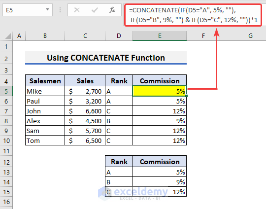
5. Use CONCATENATE Function

The SWITCH function was introduced in Excel 2016. The older versions don’t have the SWITCH function. In that case, you can use the CONCATENATE function in place of the previous method. Apply the formula in cell E5.

Here, we have concatenated multiple IF functions. This formula shows 5 % if the value of Cell D5 is A, 9 % if B, and 12 % if C.

Read More: Nested Formula with AVERAGE and ROUND Functions in Excel

Frequently Asked Questions

1. What is the limit of nested IF in Excel?

The maximum number of nested IF functions in Excel depends on the version of Excel you are using.

In Excel 2016 and later versions, the maximum number of nested IF functions is 64. This means you can nest up to 64 IF functions within a single formula.

In earlier versions of Excel, such as Excel 2013 and earlier, the maximum number of nested IF functions is 7.

2. What are the disadvantages of nested IF function?

The formula gets complicated with the application of a lot of IF blocks. It limits flexibility and increases the calculation time compared to other functions like VLOOKUP or SWITCH.

Takeaways from this Article

• The nested IF function allows you to perform more complex calculations in Excel by nesting multiple IF statements within each other.
• To use the nested IF function, you need to specify the logical test or condition that you want to evaluate, as well as the value or action to take if the condition is true or false.
• Using conditional formatting with nested IF allows highlighting cells which is more helpful in practical scenarios.
• You can combine the nested IF function with other functions in Excel, such as the AND and OR functions, to create even more complex logic and calculations.

Things to Remember

• When nesting IF functions, it’s important to ensure that each condition is properly nested and that you use the correct syntax to avoid errors.
• When using nested IF functions, it’s important to use parentheses to group each condition and its corresponding result.
• Consider other functions, such as the VLOOKUP or SWITCH functions, to see if they can simplify your formula.

Download Practice Book

Download the practice book from here.

Conclusion

So, these are all about how to use nested IF functions in Excel. In this article, we have covered several examples of how you can use the nested IF function in Excel, including finding multiple results based on criteria, finding grades, allocating vacation days, using text conditions, applying conditional formatting, and inserting logical operators (AND/OR). The most popular use of the nested IF function is finding grade. However, it’s important to keep your formula simple, use indentation and parentheses to group conditions, test the formula on a small set of data, and keep track of the number of nested levels. With these tips in mind, you can use nested IF functions in Excel and take your data analysis skills to the next level. If you have any suggestions or queries, feel free to ask in the comment section below.

<< Go Back to Nested Formula | Excel Formulas | Learn Excel