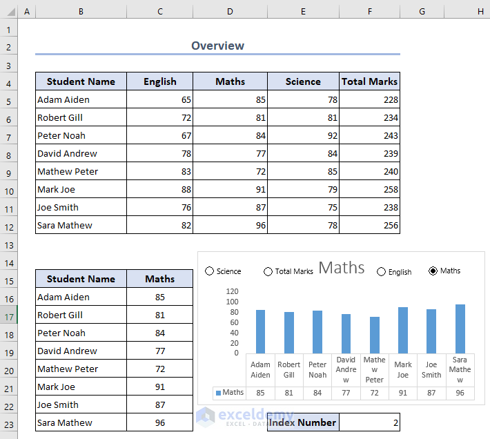
Below is an overview of our sample dataset.
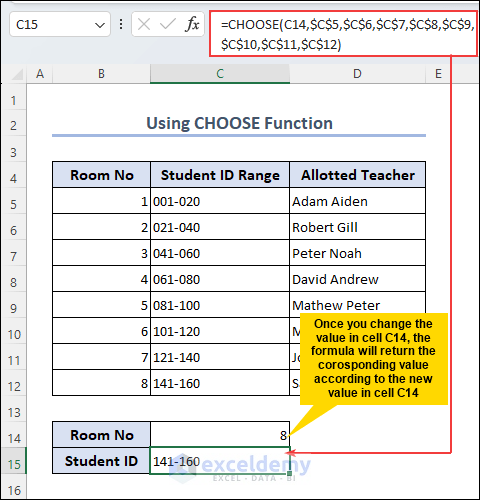
Example 1 – Using CHOOSE Function to Get Data from Selected Range
The CHOOSE function will return the value from the list at a specific position. If you select a range of student IDs and write 8, this function will return the value of the 5th position.
=CHOOSE(C14,$C$5,$C$6,$C$7,$C$8,$C$9,$C$10,$C$11,$C$12)- In this formula, cell C14 is the index number. You will get the position of the output from the index number and the rest of the cells are values to get the output as required.
Example 2 – Applying the CHOOSE Function to Get the Sum
=SUM(CHOOSE(C14,$D$5:$F$5,$D$6:$F$6,$D$7:$F$7,$D$8:$F$8,$D$9:$F$9,$D$10:$F$10,$D$11:$F$11,$D$12:$F$12))- Index number cell C14 will return the value of the nth position (till 254) and the selected ranges are the values. This function will return the sum value of the selected range according to the Index Number.
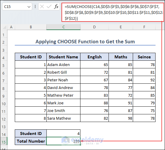
Formula Breakdown
SUM()
- The sum function sums up the lookup range used in the formula.
SUM(CHOOSE(C14,$D$5:$F$5,$D$6:$F$6,$D$7:$F$7,$D$8:$F$8,$D$9:$F$9,$D$10:$F$10,$D$11:$F$11,$D$12:$F$12))
- The CHOOSE function chooses the required value and the SUM function sums up the data as output.
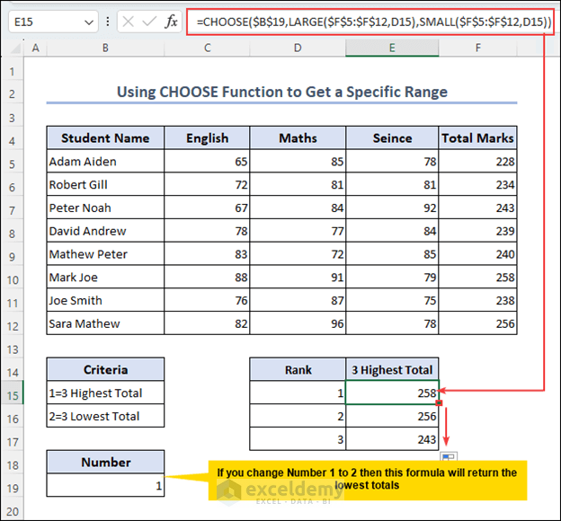
Example 3 – Using the CHOOSE Function to Get a Specific Range
- Select cell E14 to apply the formula.
=CHOOSE($B$19,"3 Highest Total","3 Lowest Total")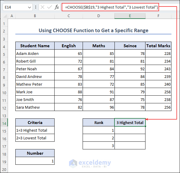
- Select cell B19 to apply for the index number and lock the cell.
- Enter the criteria and complete the formula.
- Enter another formula using the CHOOSE function, the LARGE function and the SMALL function to get the values of the selected criteria as below.
=CHOOSE($B$19,LARGE($F$5:$F$12,D15),SMALL($F$5:$F$12,D15))- Drag down the Fill handle to get all three highest or lowest values.
Formula Breakdown
SMALL($F$5:$F$12,D15)
- $F$5:$F$12 range will find out the specific value according to the index number in cell D15 and return the value as the lowest number.
LARGE($F$5:$F$12,D15)
- The range $F$5:$F$12 will find the value according to the cell D15 and return the highest marks as criteria.
CHOOSE($B$19,LARGE($F$5:$F$12,D15),SMALL($F$5:$F$12,D15))
- The CHOOSE function will return the three highest or three lowest values according to the criteria in cell B19.
Example 4 – Utilizing CHOOSE Function as a Reminder (Custom Day/Month)
- Enter the formula to get the days in cell D5.
=CHOOSE(WEEKDAY(C5),"Saturday","Sunday","Monday","Tuesday","Wednesday","Thursday","Friday")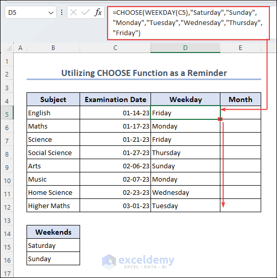
- The CHOOSE function will return the selected date and the WEEKDAYS function will return the day of the selected date.
- Get the month name with the MONTH function using the same process already used in “Weekday”.
=CHOOSE(MONTH(C5),"January","February","March","April","May","June","July","August","September","October","November","December")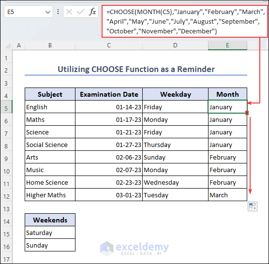
Read More: Advanced Uses of CHOOSE Function in Excel
Example 5 – Using CHOOSE Function to Get Value from Specific Lookup Range
- Select cell C15 and enter the function below.
=VLOOKUP(C14,CHOOSE({2,1}, C5:C12, B5:B12),2,FALSE)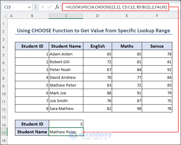
Formula Breakdown
CHOOSE({2,1}, C5:C12, B5:B12
- {2,1} shows that column C is the 2nd column and column B is the first column and CHOOSE function selects the value from these to the column.
VLOOKUP(C14,CHOOSE({2,1}, C5:C12, B5:B12),2,FALSE)
- The VLOOKUP function searches the value from the lookup range and provides the required output as shown.
Read More: How to Use VLOOKUP with CHOOSE Function in Excel
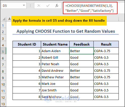
Example 6 – Applying RANDBETWEEN Function to Get Random Values
=CHOOSE(RANDBETWEEN(1,3),"Better","Good","Satisfactory")- The RANDBETWWEN function returns a random value here and the CHOOSE function chooses the value to get the required output.
Example 7 – Utilizing CHOOSE Function to Get a Specific Range from Chart
- Create a chart (go to Insert >> Chart) selecting Student ID as X-axis. and the subjects as Y-axis.
- Select cell C15 to insert the CHOOSE function to choose a specific range of data at a time in the chart.
=CHOOSE($B$26,C4,D4,E4,F4)- To apply and activate the Option Button go to Developer >> Insert >> Option Button and link the button to Index Number.
- To link the option buttons right-click the button, and choose Format Control >> Control >> Checked.
- Right down the cell name and lock the cell to complete the process.
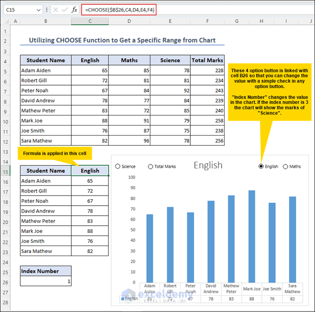
Note: Cell B26 is the index number and C4, D4, E4 and F4 are values. The value cells are not locked, drag down the formula until cell C23.
How to Use Other Functions Instead of CHOOSE Function: 2 Examples
Example 1: Using the SWITCH Function as a Reminder
- Select cell D5 and get the weekday as output.
=SWITCH(WEEKDAY(C5),1,"Saturday",2,"Sunday",3,"Monday",4,"Tuesday",5,"Wednesday",6,"Thursday",7,"Friday")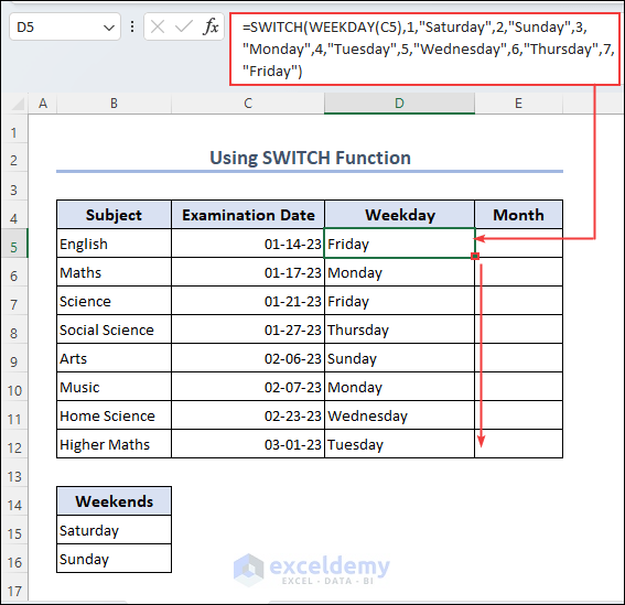
- The method of executing this process is like the earlier method but instead of using the CHOOSE function, we used the SWITCH function.
- Insert another formula in cell E5 to get the month name from the date.
=SWITCH(MONTH(C5),1,"January",2,"February",3,"March",4,"April",5,"May",6,"June",7,"July",8,"August",9,"September",10,"October",11,"November",12,"December")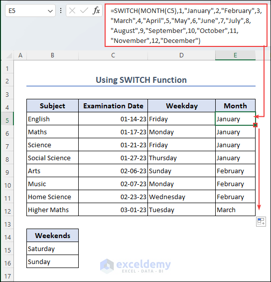
Example 2 – Applying the Nested IF Function to Get Required Value
- If the function doesn’t match the criteria, the formula will return the value as No Match otherwise the formula will return the value according to the value in cell B15.
=IF(B15>9,"NoMatch",IF(B15=8,D12,IF(B15=7,D11,IF(B15=6,D10,IF(B15=5,D9,IF(B15=4,D8,IF(B15=3,D7,IF(B15=2,D6,IF(B15=1,D5,"No Match")))))))))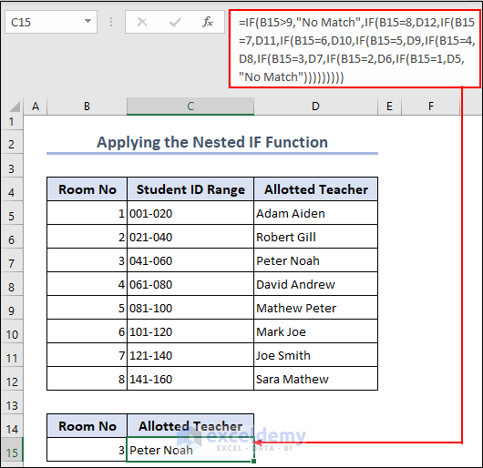
Formula Breakdown
IF(B15>9,”NoMatch”
- If the value of cell B15 is greater than 9, the output will be “No Match”.
IF(B15=8,D12
- The data will return a value as cell D12 if cell B15 is 8.
- This function will continue its loop until the value of cell B15 is 1.
IF(B15>9,”NoMatch”,IF(B15=8,D12,IF(B15=7,D11,IF(B15=6,D10,IF(B15=5,D9,IF(B15=4,D8,IF(B15=3,D7,IF(B15=2,D6,IF(B15=1,D5,”No Match”)))))))))
- This formula will return value according to the mentioned cell till the value in cell B15 is between 1-8. Otherwise, the output is “No Match”.
Read More: How to Use CHOOSE Function to Perform IF Condition in Excel
Things to Remember
- While using the CHOOSE function the index number should be always a positive whole number and should correspond to the values.
- There is a value limit in the CHOOSE function the lowest value is 1 and the highest value is 254.
Download Practice Workbook
Excel CHOOSE Function: Knowledge Hub
- How to Use CHOOSE Function with Array in Excel
- How to Apply CHOOSE Function to Create Drop-Down List in Excel
- How to Use CHOOSE Function in Excel for Scenarios
- How to Use Excel Formula to Choose Between Two Values
<< Go Back to Excel Functions | Learn Excel
Get FREE Advanced Excel Exercises with Solutions!
